Takeaways
- Understanding of the logic behind NHST
- Intuition about what power is
- See why power, perhaps, potentially isn’t just a hoop to jump through
Where it all started
Sir Ronald Fisher (1890-1962)
![]()
- Probability value = p-value
- Central question: How likely is it to observe such data if there were nothing?
The original p-value
- Tea or milk first
- How many cups would you want to be convinced?
- Correctly identifying all 8 cups: 1.4% chance to occur if the lady can’t taste the difference
- 1.4% < 5%
What’s a p-value
Informally: What’s the chance of observing something like this if there were nothing going on?
\[\begin{gather*}
Chance = (Finding \ something \ like \ this \ | \ Nothing \ going \ on)
\end{gather*}\]
Formally: The probability of observing data this extreme or more extreme under the null hypothesis
\[\begin{gather*}
P = (Data|H_0)
\end{gather*}\]
Error rates
If we’re forced to make a decision, then error rates are what we deem acceptable levels of being right/wrong in the long-run:
- \(\alpha\)
- \(\beta\)
- 1 - \(\beta\)
- 1 - \(\alpha\)
When there’s nothing
When there truly is no effect, two things can happen: We find a significant effect or we don’t.
- False positive: Saying there’s something when there’s nothing (Type I error)
- True negative: Saying there isn’t something when there is nothing. (Correct)
When there’s nothing
When there truly is no effect, two things can happen: We find a significant effect (error) or we don’t (no error).
- \(\alpha\): The probability of observing a significant result when H0 is true.
- 1 - \(\alpha\): The probability of observing a nonsignificant result when H0 is true.
When there’s something
When there truly is an effect, two things can happen: We find no significant effect (error) or we find one (correct).
- False negative: Saying there isn’t something when there’s something (Type II error)
- True positive: Saying there’s something when there’s something. (Correct)
When there’s something
When there truly is an effect, two things can happen: We find no significant effect (error) or we find one (correct).
- \(\beta\): The probability of observing a nonsignificant result when H1 is true
- 1 - \(\beta\): The probability of observing a significant result when H1 is true.
Why am I talking so weird?
“When there isn’t something?” Why not just say there’s nothing?
\[\begin{gather*}
(Data|H_0) \neq (H_0|Data)
\end{gather*}\]
We can’t find evidence for H0 with “classical” NHST (unless we use equivalence tests). A nonsignificant p-value only means we can’t reject H0, and therefore can’t accept H1, but we can’t accept H0.
Where’s our power?
| Significant |
False Positive (\(\alpha\)) |
True Positive (1-\(\beta\)) |
| Nonsignificant |
True Negative (1-\(\alpha\)) |
False negative (\(\beta\)) |
Power
Power is the probability of finding a significant result when there is an effect. It’s determined (simplified) by:
- Effect size
- Sample size
- Error rates (\(\alpha\) and \(\beta\))
Pictures, please
Let’s assume we want to know whether the population mean is larger than 50. We sample n = 100.
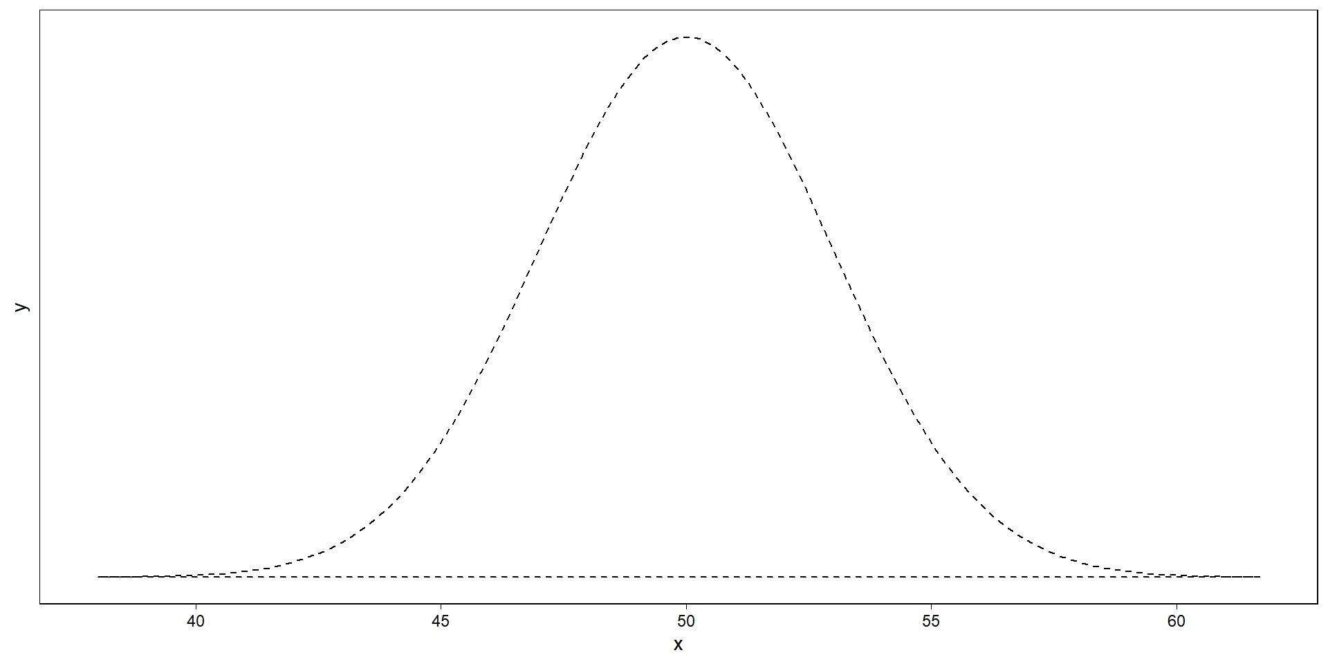
The null distribution
This is the sampling distribution if the null were true: The true effect is 50.
![]()
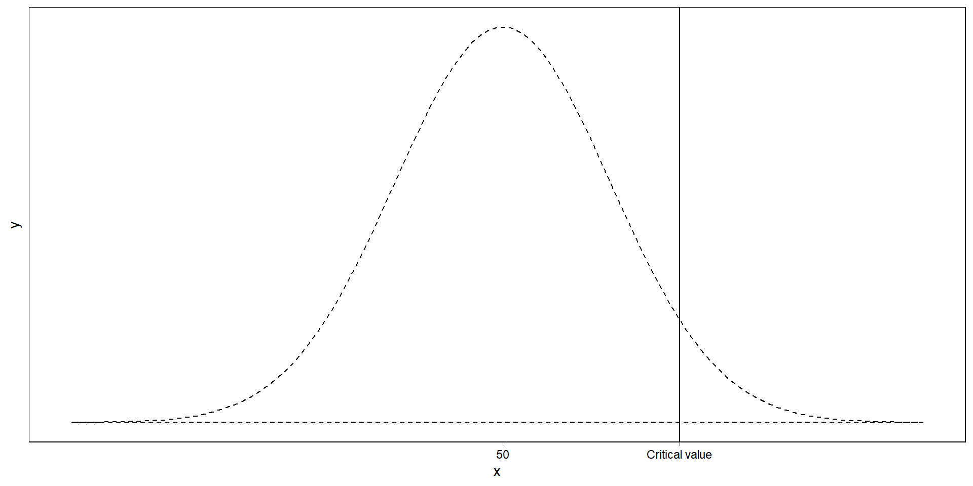
The null distribution
Where does a sample need to fall for us to wrongly conclude there’s a difference?
![]()
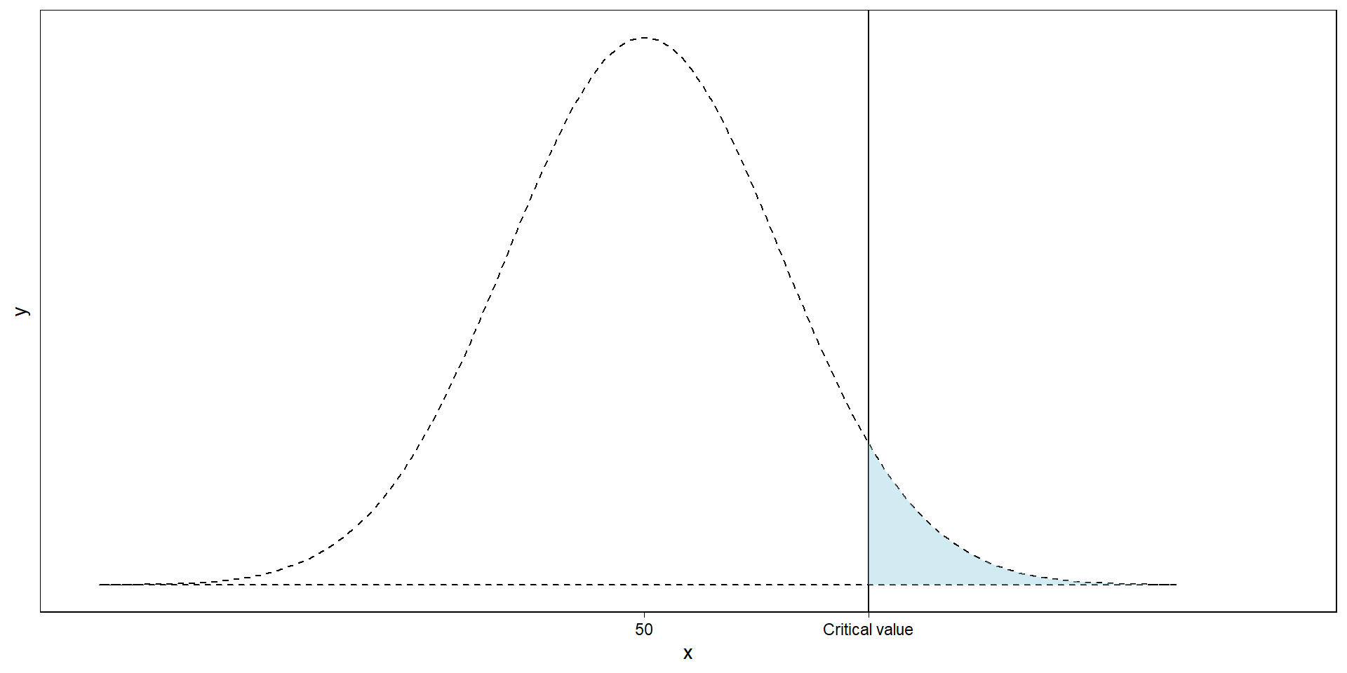
The null distribution
That’s our \(\alpha\): our false positives. Left of it: our true negatives (1-\(\alpha\)).
![]()
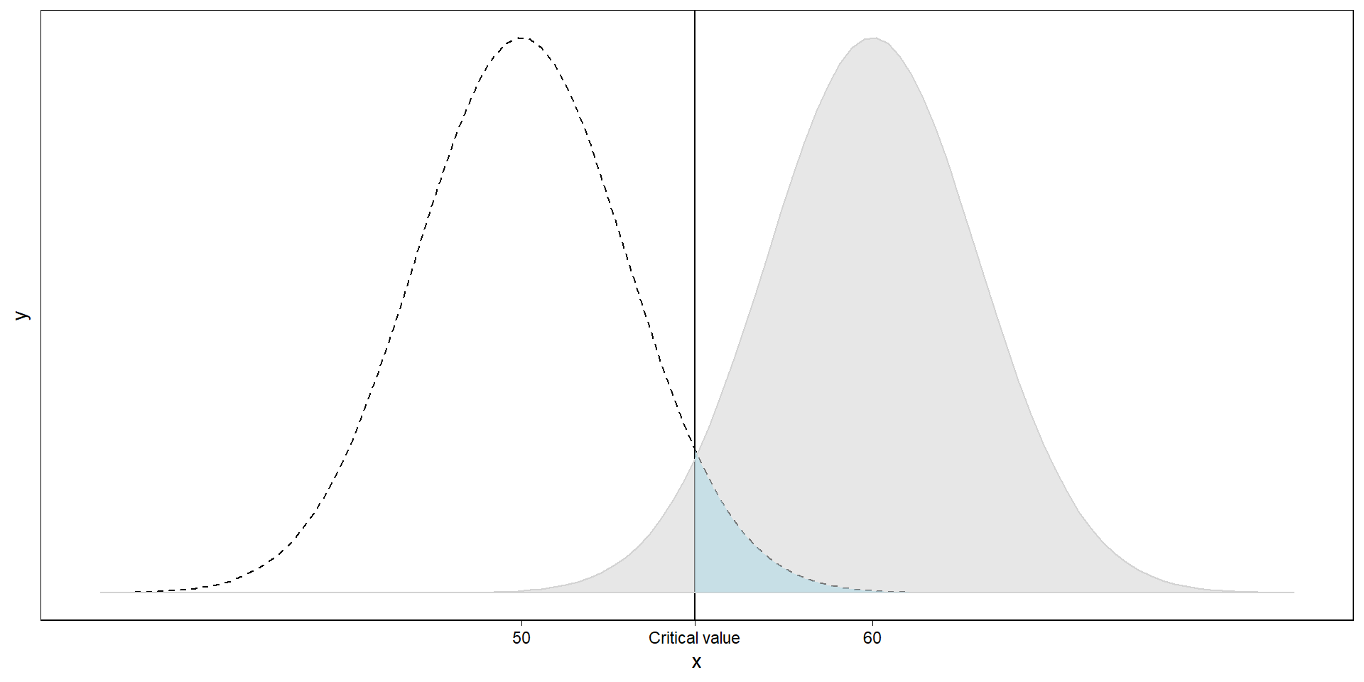
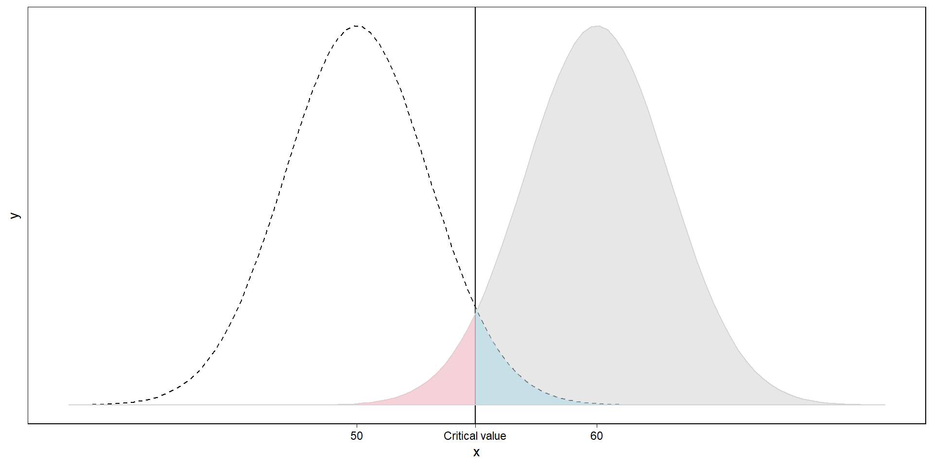
Where would we conclude it’s coming from then?
Our sampling distribution if the population value is 60. We commit a false positive if we assume a sample comes from the right distribution if in fact it comes from the left.
![]()
What about the reverse?
Our \(\beta\): our false negatives. We commit a false negative if we assume a sample comes from the left distribution if in fact it comes from the right.
![]()
Where’s power then?
![]()
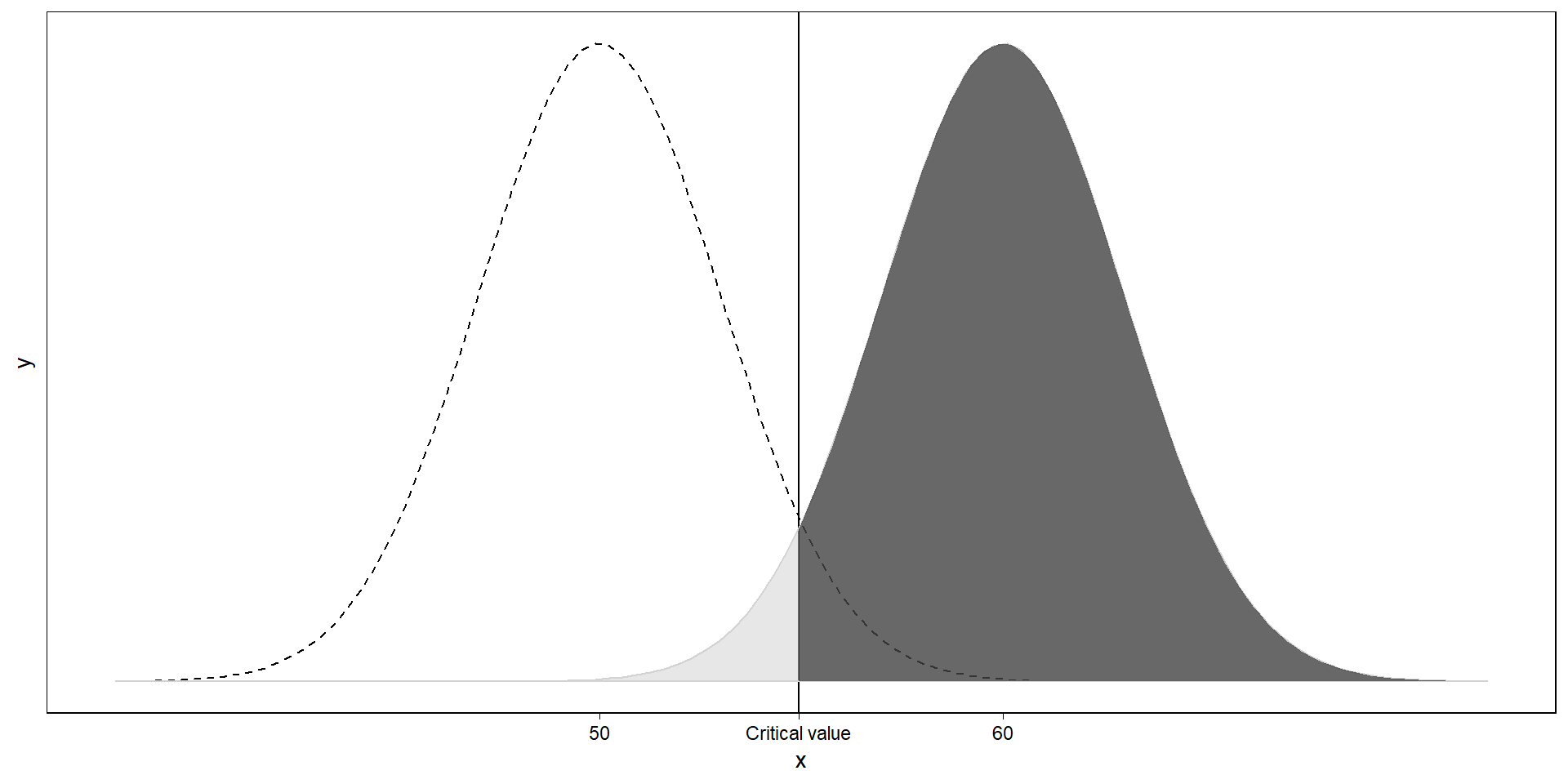
Where’s power then?
Everything right of the critical value: If a sample comes from the right distribution, this is how often we’ll correctly identify it.
![]()
What determined power again?
Power is the probability of finding a significant result when there is an effect. It’s determined (simplified) by:
- Effect size
- Sample size
- Error rates (\(\alpha\) and \(\beta\))
Let’s have a look how: Preview
Why does power matter?
Running studies with low power (aka underpowered studies) risks:
- Missing effects
- Inflating those effects we find
- Lower chance that a significant result is true
Missing effects
Society has commissioned us to find out something. Why would we start by setting us up so that we’re barely able to do that?
- Waste of resources
- Super frustrating
- Dissuades others
- Can slow down entire research lines
Inflating those effects we find
Let’s go back to our example. Let’s assume we want to know whether the population mean is larger than 50. We sample n = 100.
![]()
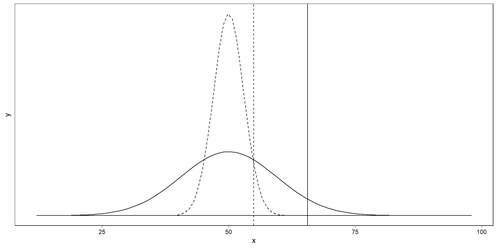
What if we sample only 10?
The sampling distribution gets wider: Now a sample mean needs to be really large to be significant. The smaller our sample (aka the lower our power), the more extreme a sample has to be to “make it” across the critical value.
![]()
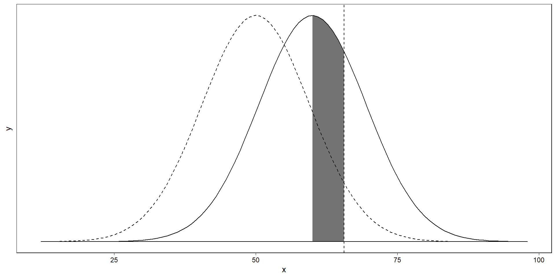
Low power inflates effects
If our study is small (has low power), only an overestimate will pass our threshold for significance. With underpowered studies, significant results will always be an overestimate. Below, even effects that are larger than the average true effect won’t be found.
![]()
Put differently
Tu put it differently: Small studies are only sensitive to large effects. But if the effect is truly small, we’ll only get a significant result for the rare massive overestimate.
Let’s have a look again: Preview
How true is a study?
How many effects will we expect?
- Probability to find an effect = power
- Odds of there being an effect = R
So:
\[\begin{gather*}
power \times R
\end{gather*}\]
How true is a study?
How many significant results do we expect?
- True effects (power x R)
- False positive
\[\begin{gather*}
power \times R + \alpha
\end{gather*}\]
Positive predictive value
What is the probability that a significant effect is indeed true? The rate of significant results that represent true effects divided by all significant results.
\[\begin{gather*}
PPV = \frac{power \times R}{power \times R + \alpha}
\end{gather*}\]
An example
Let’s assume our hypothesis has a 25% of being true and we go for the “conventional” alpha-level (5%).
\[\begin{gather*}
PPV = \frac{power \times R}{power \times R + \alpha}
= \frac{power \times \frac{P(effect)}{P(No \ effect)}}{power \times \frac{P(effect)}{P(No \ effect)} + \alpha}
\end{gather*}\]
- With 95% power and 1/4 odds?
- 86%
- With 40% power and 1/4 odds?
- 73%
What does this mean?
Bottom line: The lower our power, the lower the probability that our significant effects represent the truth. Aka: Low power produces false findings.
Why should we care?
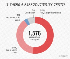
Heard of the replication crisis?
![]()
(Baker 2016)
Killer combo
- Bad research + low power
- False positives
- Inflated effect sizes
- Inflated false positives = low credibility and a waste of resources
“[The] lack of transparency in science has led to quality uncertainty, and . . . this threatens to erode trust in science” (Vazire 2017)
On the flip side
- Oversampling risks wasting resources too
- Value of information: Not every data point has the same value
- Our power should align with our inferential goals