Simulations in R

Power analysis through simulation in R

Niklas Johannes

Takeaways

• Understand why simulations are useful
• Logic of Monte Carlo Simulations
• Basic tools

Why should I simulate

• Cooking vs. eating
• Makes you truly understand what you’re doing
• Forces you to put a number on things
• Simulate the data generating process (we’ll get back to that)

Going through the motions

• You’ll often find that you don’t know nearly enough for a prediction–or even a study
• If we can’t generate the pattern we’re interested in how can we explain a pattern?
• I take a proper description over a flawed confirmation

Technicalities

Above all, you want to be able to reproduce your analysis–much later, on a different computer, etc. (Trisovic et al. 2022)

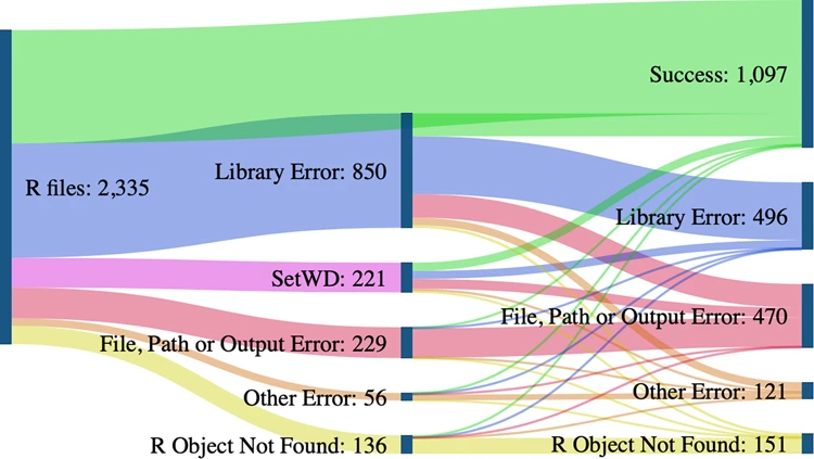
Computational reproducibility

• Environment
• Packages for project
• Packages for script
• Version control

For now

• set.seed(): Reproduce random numbers within same script
• sessionInfo(): Prints computational environment
• Relative paths (here package)
• Explicit caching or markdown

Monte Carlo simulations

Monte Carlo methods, or Monte Carlo experiments, are a broad class of computational algorithms that rely on repeated random sampling to obtain numerical results. The underlying concept is to use randomness to solve problems that might be deterministic in principle. Wikipedia

Source

In plain English

• Define relevant outcome, the process leading to outcome, and potential inputs that go into the process
• Then decide what inputs you want to vary
• Run the process many, many times, with different inputs, summarize and plot the outcomes

A simple example

Totally unrelated to why you are here:

• Outcome: How much power do I have?
• Process: The statistical test I plan to do
• Inputs: Effect size, sample size, \(\alpha\)

Some basic commands first

Sampling a certain number of elements from a set.

my_sample <- 1:20

sample(
  x = my_sample,
  size = 2
)

[1] 12  2

Sampling

With or without replacement?

my_sample <- c("a", "b", "c")

sample(
  x = my_sample,
  size = 4,
  replace = TRUE
)

[1] "b" "b" "c" "c"

On those letters

R has some neat built-in stuff.

letters[5]

[1] "e"

letters[7:10]

[1] "g" "h" "i" "j"

LETTERS[20:26]

[1] "T" "U" "V" "W" "X" "Y" "Z"

Sampling

Using those letters.

my_sample <- letters[1:3]

sample(
  x = my_sample,
  size = 4,
  replace = TRUE
)

[1] "a" "a" "b" "b"

Sampling

Assigning different probabilities.

my_sample <- c("black", "blue")

sample(
  x = my_sample,
  size = 10,
  replace = TRUE,
  prob = c(0.2, 0.8)
)

 [1] "blue" "blue" "blue" "blue" "blue" "blue" "blue" "blue" "blue" "blue"

Remember seeds?

my_sample <- c("black", "blue")

set.seed(42)
sample(
  x = my_sample,
  size = 10,
  replace = TRUE,
  prob = c(0.2, 0.8)
)

 [1] "black" "black" "blue"  "black" "blue"  "blue"  "blue"  "blue"  "blue" 
[10] "blue" 

set.seed(42)
sample(
  x = my_sample,
  size = 10,
  replace = TRUE,
  prob = c(0.2, 0.8)
)

 [1] "black" "black" "blue"  "black" "blue"  "blue"  "blue"  "blue"  "blue" 
[10] "blue" 

How do we generate randomness?

Built-in R functions that create a random number following a process with a given probability distribution.

• rnorm: Normal distribution
• rbinom: Binomial distribution
• rpois: Poissong distribution
• runif: Uniform distribution

Normal distribution

Draw n numbers from a normal distribution.

rnorm(
  n = 5,
  mean = 0,
  sd = 1
)

[1] -0.10612452  1.51152200 -0.09465904  2.01842371 -0.06271410

Once more: seed

rnorm(1)

[1] 1.30487

rnorm(1)

[1] 2.286645

set.seed(42)
rnorm(1)

[1] 1.370958

set.seed(42)
rnorm(1)

[1] 1.370958

R uses vectors

Gives us 4 draws total: 1 draw from a normal distribution with mean = 0 and sd = 1, 1 draw from a normal distribution with mean = 10 and sd = 50, and so on.

rnorm(
  n = 4,
  mean = c(0, 10, 20, 30),
  sd = c(1, 50, 100, 150)
)

[1] -0.5646982 28.1564206 83.2862605 90.6402485

What would I use this for?

Simulating different groups.

control <- 
  rnorm(
    n = 100,
    mean = 100,
    sd = 15
  )

treatment <- 
  rnorm(
    n = 100,
    mean = 150,
    sd = 15
  )

What would I use this for?

Simulating different groups.

boxplot(control, treatment)

What would I use this for?

Simulating a correlation.

control <- 
  rnorm(
    n = 1000,
    mean = 100,
    sd = 15
  )

treatment <- 
  control*0.5 + rnorm(
    n = 1000,
    mean = 100,
    sd = 15
  )

What would I use this for?

summary(lm(treatment~control))

Call:
lm(formula = treatment ~ control)

Residuals:
    Min      1Q  Median      3Q     Max 
-42.531  -9.904  -0.444  10.315  53.874 

Coefficients:
             Estimate Std. Error t value Pr(>|t|)    
(Intercept) 100.71554    3.15133   31.96   <2e-16 ***
control       0.49205    0.03129   15.72   <2e-16 ***
---
Signif. codes:  0 '***' 0.001 '**' 0.01 '*' 0.05 '.' 0.1 ' ' 1

Residual standard error: 14.86 on 998 degrees of freedom
Multiple R-squared:  0.1985,    Adjusted R-squared:  0.1977 
F-statistic: 247.2 on 1 and 998 DF,  p-value: < 2.2e-16

Teaser for later

Same data, different conventions.

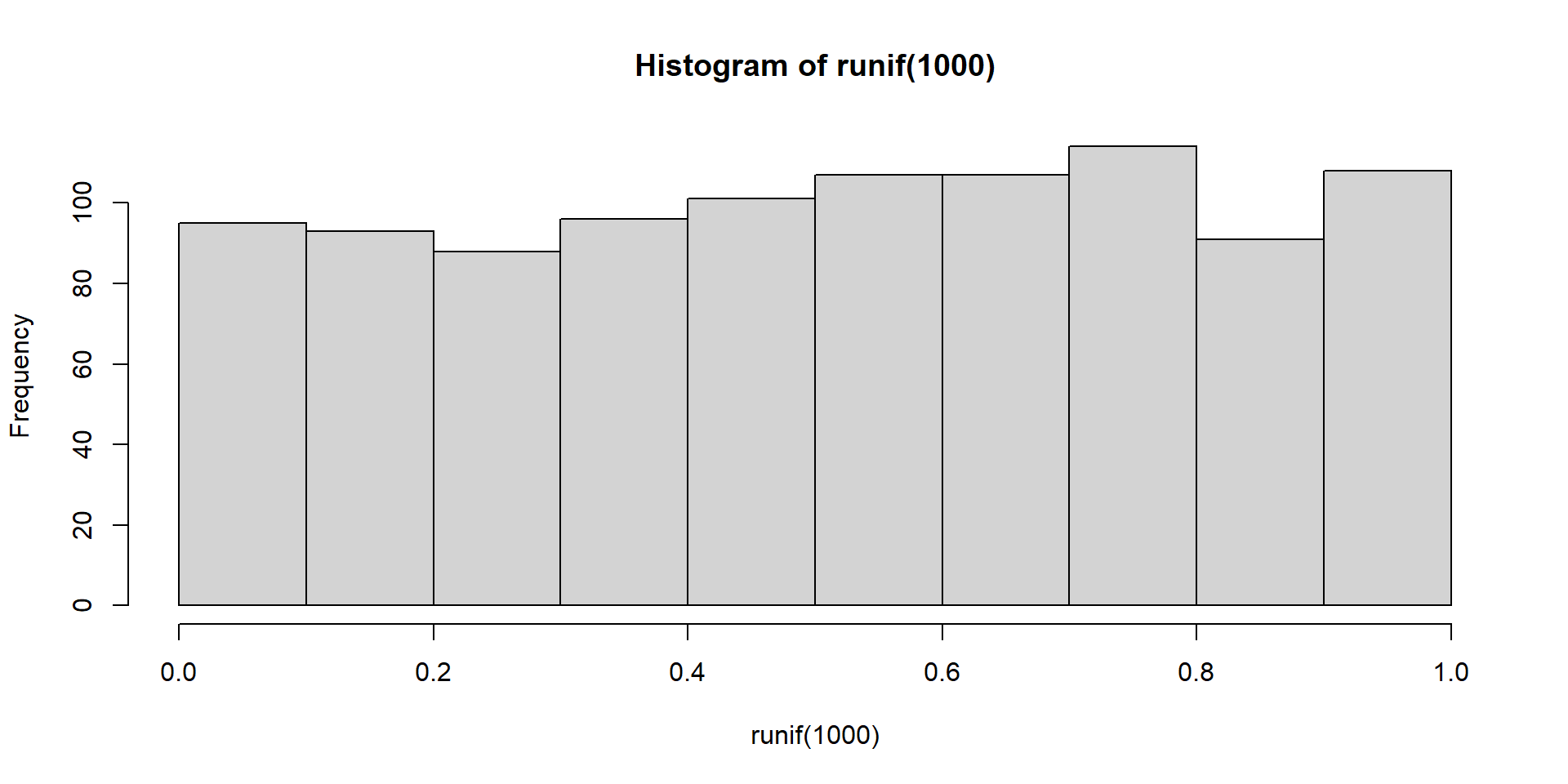
Uniform distribution

Draw n numbers from a uniform distribution.

runif(
  n = 5,
  min = 0,
  max = 1
)

[1] 0.06866080 0.05036072 0.98707779 0.63460261 0.94782652

Let’s inspect that

hist(runif(1000))

What would I use this for?

Keeping a range on predictor variables.

age <- runif(n = 1000, min = 18, max = 100)

hist(age, breaks = 30, xlim = c(18, 100))

What would I use this for?

Keeping a range on predictor variables.

age <- runif(n = 1000, min = 18, max = 100)
y <- age*0.5 + rnorm(1000)

summary(lm(y~age))

Call:
lm(formula = y ~ age)

Residuals:
    Min      1Q  Median      3Q     Max 
-3.0665 -0.6815 -0.0112  0.6320  3.4804 

Coefficients:
             Estimate Std. Error t value Pr(>|t|)    
(Intercept) -0.026915   0.082359  -0.327    0.744    
age          0.499389   0.001297 384.986   <2e-16 ***
---
Signif. codes:  0 '***' 0.001 '**' 0.01 '*' 0.05 '.' 0.1 ' ' 1

Residual standard error: 0.9858 on 998 degrees of freedom
Multiple R-squared:  0.9933,    Adjusted R-squared:  0.9933 
F-statistic: 1.482e+05 on 1 and 998 DF,  p-value: < 2.2e-16

Binomial distribution

Let’s flip a coin 100 times. That’s one “experiment”. How often will I get heads?

rbinom(
  n = 1,
  size = 100,
  prob = 0.50
)

[1] 43

Many experiments

Let’s run 1000 experiments where we flip a coin 100 times each.

experiments <- 
  rbinom(
    n = 1000,
    size = 100,
    prob = 0.50
  )

head(experiments)

[1] 46 56 49 48 53 58

Always inspect and summarize

Makes sense.

hist(experiments, breaks = 20)

What would I use this for?

Compare groups on their probabilities.

control <- 
  rbinom(
    n = 100,
    size = 10,
    prob = 0.5
  )

treatment <- 
  rbinom(
    n = 100,
    size = 10,
    prob = 0.9
  )

What would I use this for?

Compare groups on their probabilities.

boxplot(control, treatment)

What would I use this for?

Bernoulli trials.

rbinom(
  n = 10,
  size = 1,
  prob = 0.5
)

 [1] 1 0 0 1 0 0 1 0 1 0

What would I use this for?

Bernoulli trials and logistic regression: Does age predict our binary outcome? (Explanation here.)

age <- rnorm(n = 10000, mean = 50, sd = 15)

xb <- 1 + 0.2*age

p <- 1/(1 + exp(-xb))

y <- 
  rbinom(
    n = 10000,
    size = 1,
    prob = p
  )

What would I use this for?

m <- 
  glm(
    y ~ age,
    family = binomial()
  )

summary(m)

Call:
glm(formula = y ~ age, family = binomial())

Deviance Residuals: 
    Min       1Q   Median       3Q      Max  
-3.6531   0.0002   0.0011   0.0047   1.0001  

Coefficients:
            Estimate Std. Error z value Pr(>|z|)    
(Intercept)  0.13900    0.56322   0.247    0.805    
age          0.28512    0.04927   5.787 7.18e-09 ***
---
Signif. codes:  0 '***' 0.001 '**' 0.01 '*' 0.05 '.' 0.1 ' ' 1

(Dispersion parameter for binomial family taken to be 1)

    Null deviance: 171.86  on 9999  degrees of freedom
Residual deviance:  66.03  on 9998  degrees of freedom
AIC: 70.03

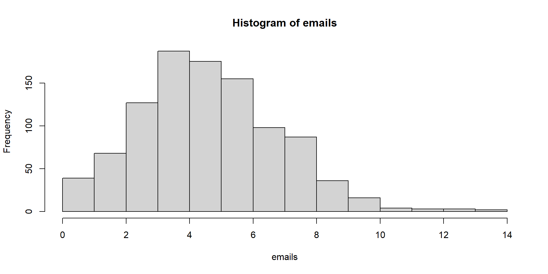
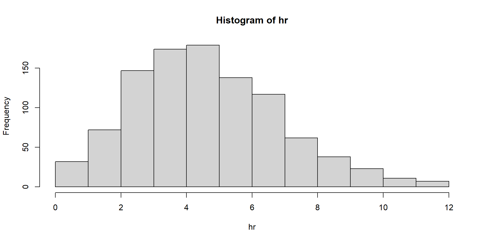
Number of Fisher Scoring iterations: 13

Poisson distribution

Let’s see how many emails we get in an hour. We check for 10 different hours.

rpois(
  n = 10,
  lambda = 5
)

 [1] 3 4 5 2 8 5 7 5 5 5

Let’s visualize

emails <- 
  rpois(
    n = 1000,
    lambda = 5
  )

hist(emails)

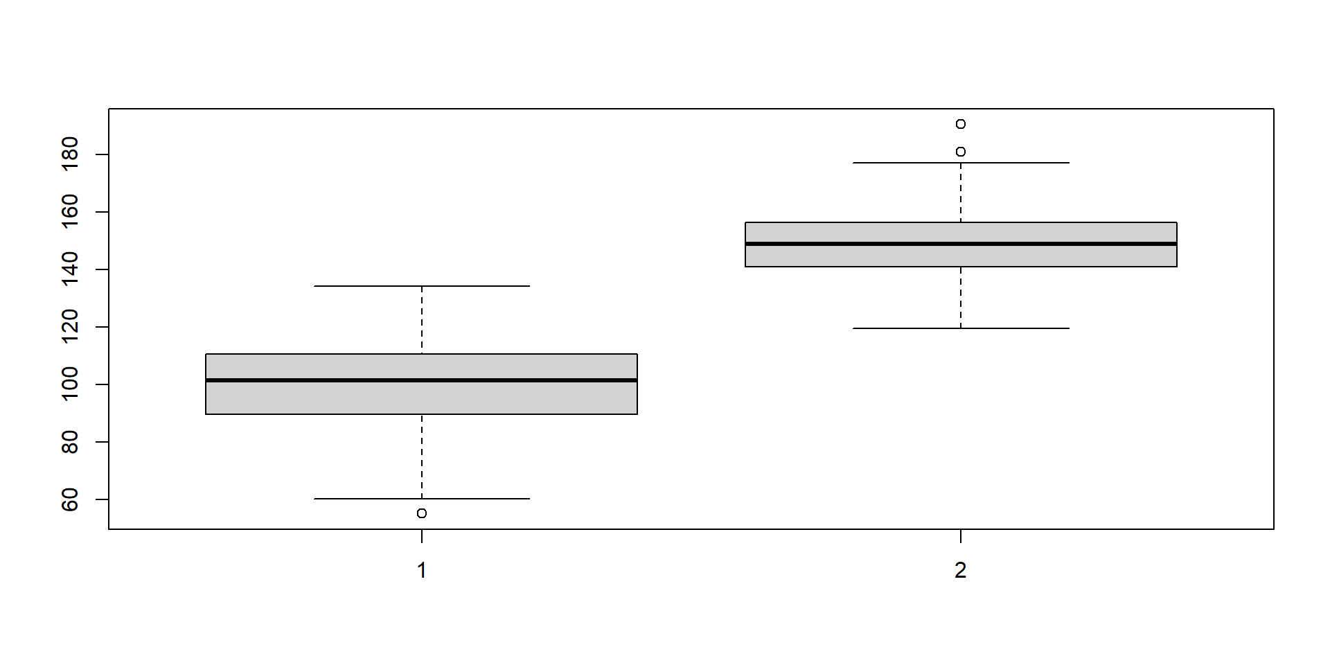
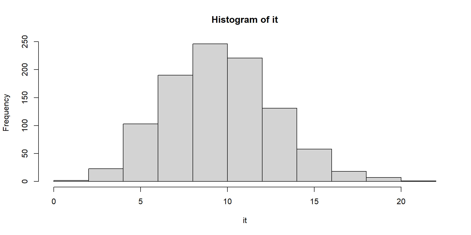
Why would you use this?

Compare two groups on how many emails they get.

hr <- rpois(n = 1000, lambda = 5)
it <- rpois(n = 1000, lambda = 10)

hist(hr)

hist(it)

What would I use this for?

Poisson regression. (More on rep in a moment.)

d <- 
  data.frame(
    emails = c(hr, it),
    group = factor(rep(c("HR", "IT"), each = 1000))
  )

d[c(1:5, 1001:1005),]

     emails group
1         5    HR
2         7    HR
3         4    HR
4         8    HR
5         2    HR
1001     10    IT
1002      9    IT
1003      5    IT
1004      6    IT
1005      7    IT

What would I use this for?

m <- 
  glm(
    emails ~ group,
    data = d,
    family = poisson()
  )

summary(m)

Call:
glm(formula = emails ~ group, family = poisson(), data = d)

Deviance Residuals: 
    Min       1Q   Median       3Q      Max  
-3.6837  -0.6850  -0.0559   0.5814   2.9916  

Coefficients:
            Estimate Std. Error z value Pr(>|z|)    
(Intercept)  1.63433    0.01397  117.01   <2e-16 ***
groupIT      0.67791    0.01715   39.53   <2e-16 ***
---
Signif. codes:  0 '***' 0.001 '**' 0.01 '*' 0.05 '.' 0.1 ' ' 1

(Dispersion parameter for poisson family taken to be 1)

    Null deviance: 3652.0  on 1999  degrees of freedom
Residual deviance: 1998.5  on 1998  degrees of freedom
AIC: 9517.7

Number of Fisher Scoring iterations: 4

Making data sets with rep

Replicates numbers and characters.

rep(
  x = "Control Group",
  times = 3
  )

[1] "Control Group" "Control Group" "Control Group"

rep(
  x = 1,
  times = 3
  )

[1] 1 1 1

Making data sets with rep

Replicates an entire vector several times.

rep(
  x = c("Control Group", "Treatment Group"),
  times = 3
  )

[1] "Control Group"   "Treatment Group" "Control Group"   "Treatment Group"
[5] "Control Group"   "Treatment Group"

Making data sets with rep

Replicate different elements different times.

rep(
  x = c("Control Group", "Treatment Group"),
  times = c(1,2)
  )

[1] "Control Group"   "Treatment Group" "Treatment Group"

Making data sets with rep

Replicates an entire vector several times.

rep(
  x = c("Control Group", "Treatment Group"),
  each = 3
  )

[1] "Control Group"   "Control Group"   "Control Group"   "Treatment Group"
[5] "Treatment Group" "Treatment Group"

Making data sets with rep

Controlling the length of our output.

rep(
  x = c("Control Group", "Treatment Group"),
  each = 3,
  length.out = 4
  )

[1] "Control Group"   "Control Group"   "Control Group"   "Treatment Group"

Making data sets with rep

Combining times with each.

rep(
  x = c("Control Group", "Treatment Group"),
  each = 3,
  times = 2
  )

 [1] "Control Group"   "Control Group"   "Control Group"   "Treatment Group"
 [5] "Treatment Group" "Treatment Group" "Control Group"   "Control Group"  
 [9] "Control Group"   "Treatment Group" "Treatment Group" "Treatment Group"

What would I use this for?

Let’s create a group.

condition <- rep("control", times = 4)
outcome <- rnorm(4)
d <- data.frame(condition, outcome)
d

  condition     outcome
1   control -0.04723942
2   control -0.12307634
3   control  1.11130209
4   control  1.07619064

What would I use this for?

Let’s create two groups.

condition <- rep(c("control", "treatment"), each = 2)
outcome <- rnorm(4)
d <- data.frame(condition, outcome)
d

  condition       outcome
1   control  0.0313900684
2   control  0.0001993327
3 treatment -0.7676236790
4 treatment  0.8964049160

Interlude: First short exercises

Different groups

Two groups from different distributions.

control_outcome <- rnorm(5, 100, 15)
treatment_outcome <- rnorm(5, 115, 15)

d <- data.frame(outcome = c(control_outcome, treatment_outcome))

Different groups

Now we add group membership.

control_outcome <- rnorm(5, 100, 15)
treatment_outcome <- rnorm(5, 115, 15)
condition <- rep(c("control", "treatment"), each = 5)


d <- data.frame(
  condition = condition,
  outcome = c(control_outcome, treatment_outcome)
)
d

   condition   outcome
1    control 102.60947
2    control 105.91958
3    control 140.17591
4    control  89.69311
5    control  94.72799
6  treatment 122.12078
7  treatment 120.31591
8  treatment 118.34136
9  treatment  91.22117
10 treatment  94.38544

Remember vectors?

Gets us there faster.

d <- 
  data.frame(
    condition = rep(c("control", "treatment"), times = 5),
    outcome = rnorm(10, mean = c(100, 115), sd = 15)
  )
d

   condition   outcome
1    control  88.88867
2  treatment 118.51307
3    control  98.56411
4  treatment  99.00802
5    control  75.87184
6  treatment 129.97625
7    control  91.31636
8  treatment 120.37524
9    control  94.46493
10 treatment 125.81974

Now how do we get to Monte Carlo?

Creating one “data set” isn’t enough. We need many more.

replicate(
  n = 5,
  expr = sample(1:4, size = 2),
  simplify = FALSE
)

[[1]]
[1] 1 3

[[2]]
[1] 3 4

[[3]]
[1] 1 3

[[4]]
[1] 2 3

[[5]]
[1] 3 2

Replicating variables

Creating one “data set” isn’t enough. We need many more.

replicate(
  n = 5,
  expr = rnorm(5),
  simplify = FALSE
)

[[1]]
[1] -1.24072975 -0.13173024  1.39906593  0.08828747  0.40500180

[[2]]
[1]  0.3126241 -0.1319878  0.4697315  0.4992376 -0.6715315

[[3]]
[1] -0.2262588 -0.1617954 -1.3745364 -1.1833134  0.8182783

[[4]]
[1]  1.2439504  1.5819136  0.6209595 -1.4514988  1.3820336

[[5]]
[1] -0.3496984  0.5724784  2.2198495 -1.2908316 -1.5562072

Replicating data sets

Creating one “data set” isn’t enough. We need more.

replicate(
  n = 5,
  expr = data.frame(
    condition = rep(c("control", "treatment"), each = 2),
    outcome = rnorm(4, c(100, 115), sd = 15)
  ),
  simplify = FALSE
)

[[1]]
  condition   outcome
1   control  86.38442
2   control 144.21596
3 treatment 100.04792
4 treatment 112.80507

[[2]]
  condition  outcome
1   control 113.5496
2   control 114.7502
3 treatment 101.7030
4 treatment 127.2264

[[3]]
  condition   outcome
1   control 128.53812
2   control 119.93447
3 treatment  99.95619
4 treatment 102.77010

[[4]]
  condition   outcome
1   control  92.93538
2   control 112.54882
3 treatment  99.87659
4 treatment 120.94084

[[5]]
  condition   outcome
1   control  60.82896
2   control 110.58693
3 treatment 119.18822
4 treatment 126.65385

for loops

For each element in a vector, do the following:

for (variable in vector) {
  
}

for (i in 1:10) {
  print(i)
}

[1] 1
[1] 2
[1] 3
[1] 4
[1] 5
[1] 6
[1] 7
[1] 8
[1] 9
[1] 10

Same as replicate

Five times we sample and store it in a list. Equivalent to replicate example.

outcome <- NULL

for (i in 1:5) {
  outcome[[i]] <- sample(1:4, size = 2)
}

outcome

[[1]]
[1] 3 2

[[2]]
[1] 1 2

[[3]]
[1] 1 2

[[4]]
[1] 4 3

[[5]]
[1] 1 4

Get our data sets

datasets <- NULL

for (i in 1:5) {
  datasets[[i]] <- 
    data.frame(
      condition = rep(c("control", "treatment"), each = 2),
      outcome = rnorm(4, c(100, 115), sd = 15)
    )
}

datasets

[[1]]
  condition   outcome
1   control  97.99421
2   control 111.00762
3 treatment  99.06100
4 treatment  81.91246

[[2]]
  condition  outcome
1   control 113.0777
2   control 126.1959
3 treatment 102.3874
4 treatment 104.5351

[[3]]
  condition   outcome
1   control 123.36611
2   control 134.27978
3 treatment  70.14792
4 treatment 112.37140

[[4]]
  condition   outcome
1   control 103.39652
2   control 119.44954
3 treatment  81.99905
4 treatment  97.97151

[[5]]
  condition  outcome
1   control 112.8112
2   control 119.5977
3 treatment 112.1696
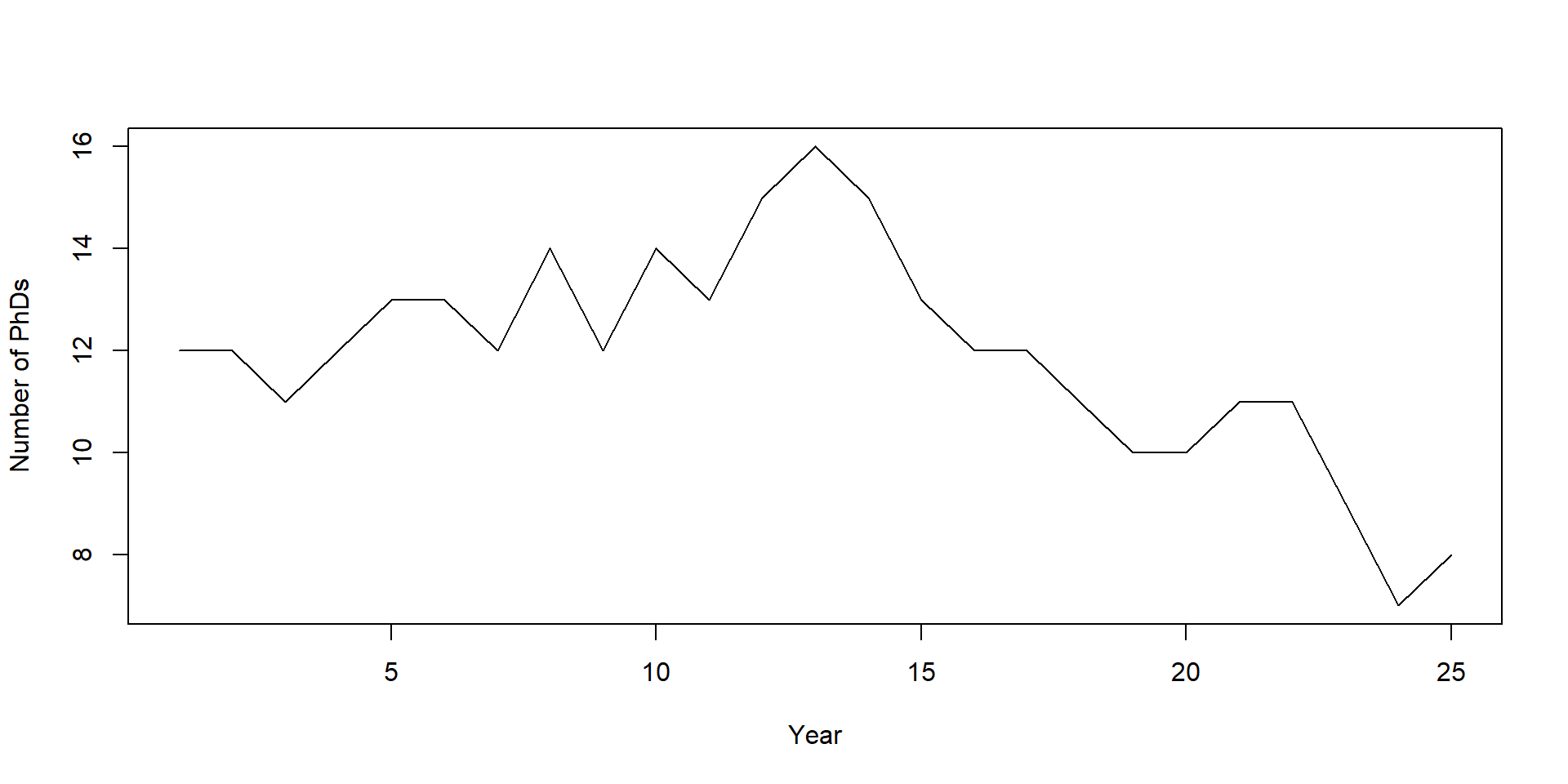
4 treatment 113.9696

A concrete example

Let’s model the growth of our department. This year, we have 12 PhD students. Each year, our 4 professors write one grant application each. If they get the money, they’ll hire one new PhD student. Their chance of getting the money is 15%. But academia also sucks sometimes, so each PhD student each year has a 5% chance of quitting and finally doing something with their lives. How large is the department after 25 years?

Let’s put that into numbers

starting <- 12
profs <- 4
money <- 0.15
quitting <- 0.05
years <- 25
results <- NULL
results[1] <- starting

Into a loop

set.seed(42)
for (current_year in 2:years) {
  # how many new phds (15% chance in 4 "trials")
  newbies <- rbinom(n = 1, size = profs, prob = money)
  
  # how many see the light and quit
  enlightened <- rbinom(n = 1, size = results[current_year  - 1], prob = quitting)
  
  # new total
  results[current_year] <- results[current_year - 1] + newbies - enlightened
  
  cat("Current year:", current_year, "Newbies:", newbies, "Enlightened:", enlightened, "Total:", results[current_year], "\n")
}

Current year: 2 Newbies: 2 Enlightened: 2 Total: 12 
Current year: 3 Newbies: 0 Enlightened: 1 Total: 11 
Current year: 4 Newbies: 1 Enlightened: 0 Total: 12 
Current year: 5 Newbies: 1 Enlightened: 0 Total: 13 
Current year: 6 Newbies: 1 Enlightened: 1 Total: 13 
Current year: 7 Newbies: 0 Enlightened: 1 Total: 12 
Current year: 8 Newbies: 2 Enlightened: 0 Total: 14 
Current year: 9 Newbies: 0 Enlightened: 2 Total: 12 
Current year: 10 Newbies: 2 Enlightened: 0 Total: 14 
Current year: 11 Newbies: 0 Enlightened: 1 Total: 13 
Current year: 12 Newbies: 2 Enlightened: 0 Total: 15 
Current year: 13 Newbies: 3 Enlightened: 2 Total: 16 
Current year: 14 Newbies: 0 Enlightened: 1 Total: 15 
Current year: 15 Newbies: 0 Enlightened: 2 Total: 13 
Current year: 16 Newbies: 0 Enlightened: 1 Total: 12 
Current year: 17 Newbies: 1 Enlightened: 1 Total: 12 
Current year: 18 Newbies: 0 Enlightened: 1 Total: 11 
Current year: 19 Newbies: 0 Enlightened: 1 Total: 10 
Current year: 20 Newbies: 0 Enlightened: 0 Total: 10 
Current year: 21 Newbies: 2 Enlightened: 1 Total: 11 
Current year: 22 Newbies: 0 Enlightened: 0 Total: 11 
Current year: 23 Newbies: 0 Enlightened: 2 Total: 9 
Current year: 24 Newbies: 0 Enlightened: 2 Total: 7 
Current year: 25 Newbies: 1 Enlightened: 0 Total: 8 

Plot and summarize the results

mean(results)

[1] 11.92

plot(results, type = "l", xlab = "Year", ylab = "Number of PhDs")

Let’s repeat those repetitions

Let’s run the above simulation several times: a loop in a loop.

set.seed(42)

experiments <- 3
outcomes <- list()

for (i in 1:experiments) {
  
  results <- NULL
  results[1] <- starting
  
  for (current_year in 2:years) {
    # how many new phds (15% chance in 4 "trials")
    newbies <- rbinom(n = 1, size = profs, prob = money)
    
    # how many see the light and quit
    enlightened <- rbinom(n = 1, size = results[current_year - 1], prob = quitting)
    
    # new total
    results[current_year] <- results[current_year - 1] + newbies - enlightened
    
    # store in overall outcomes
    outcomes[[i]] <- results
  }
}

What did we just do?

# what we created
outcomes

[[1]]
 [1] 12 12 11 12 13 13 12 14 12 14 13 15 16 15 13 12 12 11 10 10 11 11  9  7  8

[[2]]
 [1] 12 13 13 12 11 12 12 10 11 12 11 12 12 12 11 11 11 12 11 12 12 12 13 11 12

[[3]]
 [1] 12 12 12 13 13 13 13 14 14 15 15 15 15 15 15 16 15 14 15 14 14 15 15 15 14

# the means per "experiment"
lapply(outcomes, mean)

[[1]]
[1] 11.92

[[2]]
[1] 11.72

[[3]]
[1] 14.12

Let’s have a look

# the mean of the means
mean(sapply(outcomes, mean))

[1] 12.58667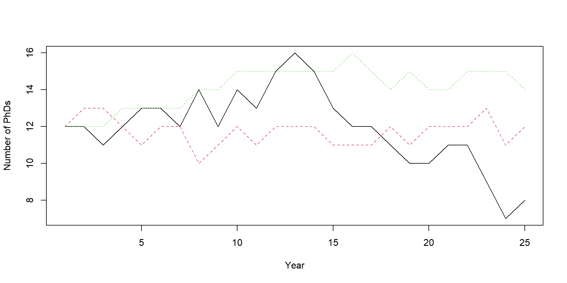

matplot(matrix(unlist(outcomes), ncol = 3), type = "l", xlab = "Year", ylab = "Number of PhDs")

What if we want to change stuff?

If we want to quickly change a parameter, it makes sense to turn this all into a function.

counting_phds <- 
  function(
    starting = 12,
    profs = 4,
    money = 0.15,
    quitting = 0.05,
    years = 25
  ) {
    
    # create our output vector
    results <- NULL
    results[1] <- starting
    
    # then our loop
    for (current_year in 2:years) {
      # how many new phds
      newbies <- rbinom(n = 1, size = profs, prob = money)
      
      # how many see the light and quit
      enlightened <- rbinom(n = 1, size = results[current_year - 1], prob = quitting)
      
      # new total
      results[current_year] <- results[current_year - 1] + newbies - enlightened
    }
    
    return(results)
  }

Let’s call that function

Now we can change parameters of the “experiment” as we wish.

counting_phds()

 [1] 12 12 10 10 11 12 12 12 11 13 14 15 15 15 16 15 15 15 15 15 15 15 16 16 15

counting_phds(profs = 10)

 [1] 12 12 12 13 14 16 18 17 20 21 21 22 21 22 22 23 21 20 21 21 22 23 26 23 24

counting_phds(years = 10)

 [1] 12 11 11 12 12 10 10 10  9  9

counting_phds(quitting = 0)

 [1] 12 13 14 15 15 15 17 17 17 18 18 20 21 21 22 22 22 23 23 23 23 23 23 23 23

Running experiments one more time

We can do the loop in a loop again, but this time we just call the function.

set.seed(42)

experiments <- 3
outcomes <- list()

for (i in 1:experiments) {
  
  # run one experiment and store the results
  results <- counting_phds()
  
  # put results into our outcomes
  outcomes[[i]] <- results

}

outcomes

[[1]]
 [1] 12 12 11 12 13 13 12 14 12 14 13 15 16 15 13 12 12 11 10 10 11 11  9  7  8

[[2]]
 [1] 12 13 13 12 11 12 12 10 11 12 11 12 12 12 11 11 11 12 11 12 12 12 13 11 12

[[3]]
 [1] 12 12 12 13 13 13 13 14 14 15 15 15 15 15 15 16 15 14 15 14 14 15 15 15 14

Combining it all

Now we can iterate (aka loop) over different arguments of our experiment. Let’s see what happens if we run 3 experiments, each with a different number of profs. We’ll store the total at the end of the time period for each run.

set.seed(42)

experiments <- 3
profs <- 4
years <- 10
outcomes <- data.frame(
  experiment = NULL,
  prof = NULL,
  total = NULL
)

for (i in 1:experiments) {
  
  # for each run/experiment, we store the results for each number of professors
  for (aprof in 1:profs) {
    results <- counting_phds(profs = aprof, years = years)
    
    # get the total at the last year
    total <- results[years]
    
    # turn into a row and add to outcomes
    our_row <- data.frame(experiment = i, prof = aprof, total = total)
    outcomes <- rbind(outcomes, our_row)
  }
}

Let’s plot

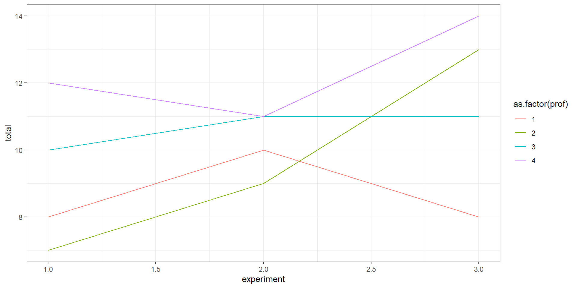
Now let’s expand

set.seed(42)

experiments <- 1000
profs <- 4
years <- 10
outcomes <- data.frame(
  experiment = NULL,
  prof = NULL,
  total = NULL
)

for (i in 1:experiments) {
  
  # for each run/experiment, we store the results for each number of professors
  for (aprof in 1:profs) {
    results <- counting_phds(profs = aprof, years = years)
    
    # get the total at the last year
    total <- results[years]
    
    # turn into a row and add to outcomes
    our_row <- data.frame(experiment = i, prof = aprof, total = total)
    outcomes <- rbind(outcomes, our_row)
  }
}

Let’s summarize and plot

With those parameters, does it make sense to have more profs?

  Group.1      x
1       1  8.630
2       2  9.750
3       3 10.819
4       4 12.023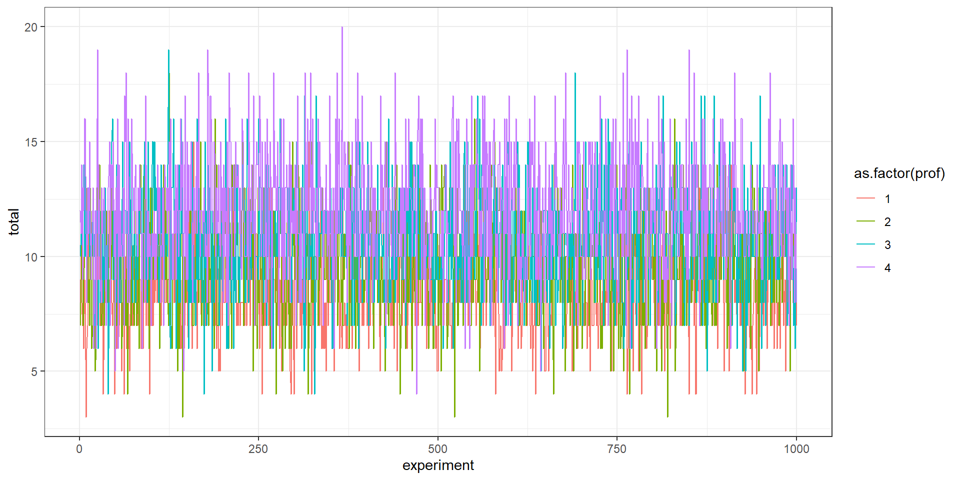

A note on efficiency

Right now, we’re appending our data to an object that grows with each iteration:

# turn into a row and add to outcomes
our_row <- data.frame(experiment = i, prof = aprof, total = total)
outcomes <- rbind(outcomes, our_row)

This procedure helps with explaining the logic, but is inefficient. It’s much faster to pre-allocate space:

outcomes <- 
  data.frame(
    experiment = rep(1:years, each = profs),
    prof = rep(1:profs, times = years),
    total = NA
  )

outcomes$total[i] <- total

For your own simulations, when efficiency matters, you should always pre-allocate space.

Let’s get simulating

References

Trisovic, Ana, Matthew K. Lau, Thomas Pasquier, and Mercè Crosas. 2022. “A Large-Scale Study on Research Code Quality and Execution.” Scientific Data 9 (1): 60. https://doi.org/10.1038/s41597-022-01143-6.