Effect sizes

Power analysis through simulation in R

Niklas Johannes

Takeaways

  • Understand the importance of effect sizes
  • How to formulate a smallest effect size of interest
  • Know when you don’t have enough information

What’s an effect size

Source

An example

Age predicts grumpiness with a large effect. But the sample is too small for significance.

set.seed(1)
age <- runif(10, 20, 80)
grumpiness <- 50 + 0.5 * age + rnorm(10, 0, 20)

cor.test(age, grumpiness)

    Pearson's product-moment correlation

data:  age and grumpiness
t = 1.5624, df = 8, p-value = 0.1568
alternative hypothesis: true correlation is not equal to 0
95 percent confidence interval:
 -0.2100550  0.8533538
sample estimates:
      cor 
0.4835198 

An example, this time larger

Age predicts grumpiness with a super tiny effect, but we have a sample of a million, so the effect is significant.

age <- runif(1e6, 20, 80)
grumpiness <- 50 + 0.01 * age + rnorm(1e6, 0, 20)

cor.test(age, grumpiness)

    Pearson's product-moment correlation

data:  age and grumpiness
t = 8.5288, df = 999998, p-value < 2.2e-16
alternative hypothesis: true correlation is not equal to 0
95 percent confidence interval:
 0.006568625 0.010488268
sample estimates:
        cor 
0.008528479 

An example, this time null

Age doesn’t predict grumpiness. Can a nonsignificant p-value tell us that?

age <- runif(1e6, 20, 80)
grumpiness <- 50 + 0 * age + rnorm(1e6, 0, 20)

cor.test(age, grumpiness)

    Pearson's product-moment correlation

data:  age and grumpiness
t = 0.093827, df = 999998, p-value = 0.9252
alternative hypothesis: true correlation is not equal to 0
95 percent confidence interval:
 -0.001866138  0.002053791
sample estimates:
         cor 
9.382711e-05 

Problems with NHST

  1. Doesn’t answer what we want to know
  2. There’ll always be a difference
  3. Nothing special about p = 0.05

Not what we want to know

Remember \(P(data|H)\), not \(P(H|data)\)?

  • We want to know how probable our hypothesis is
  • P-values don’t do that
  • Wrong focus on significance

The typical H0 is unrealistic

  • Meehl (1991): Everything in the social sciences correlates with everything
  • So-called “crud factor” (Orben and Lakens 2019)
  • With large enough samples, anything will be significant

Significant, but trivial

(Lantz 2013)

What’s so special about 0.05?

“…If one in twenty does not seem high enough odds, we may, if we prefer it, draw the line at one in fifty or one in a hundred. Personally, the writer prefers to set a low standard of significance at the 5 per cent point, and ignore entirely all results which fails to reach this level. A scientific fact should be regarded as experimentally established only if a properly designed experiment rarely fails to give this level of significance.”

(Fisher 1926)

What are we claiming?

  • Significance threshold = arbitrary
  • Evidential strength clearing that threshold = arbitrary

How not to do it

We have three independent groups: control, treatment A, and treatment B. The pesky ethics board asks us to do a power analysis. You head to GPower.

Thankfully, there’s a previous study! It had n = 20 per condition and the conditions are only somewhat similar to our planned experiment, but they do report an effect size: \(\eta_2 = .21\). Off to GPower!

Why this this approach isn’t ideal

  • No idea what \(\eta_2 = .21\) means: Is that a lot?
  • There’s three groups: What’s the effect size for?
  • Can I trust the previous study?

Let’s simulate that “previous study”

set.seed(42)
d <- data.frame(
  id = 1:60,
  condition = rep(c("control", "Treatment A", "Treatment B"), times = 20),
  score = rnorm(60, mean = c(0, 10, 20), sd = 15)
)

model <- 
  aov(
    score ~ condition, data = d
  )

effectsize::eta_squared(model)
# Effect Size for ANOVA

Parameter | Eta2 |       95% CI
-------------------------------
condition | 0.21 | [0.06, 1.00]

- One-sided CIs: upper bound fixed at [1.00].

Notice something?

Wrong rituals

  • Using effect sizes like this will get us nowhere
  • Rituals and rules of thumbs get in the way of understanding
  • But effect sizes might well be the most important part of our research

Where it all began

Cohen (1988)

Types of effect sizes

  1. Differences between groups (e.g., Cohen’s \(d\))
  2. Strength of association (e.g., Pearson’s \(r\), \(R^2\), \(\eta^2\))
  3. Estimates of risks (e.g., relative risks, odds ratios)

Differences

  • Express difference between groups in variance units, not raw units
  • Not “How many cm is the difference in height between the groups”
  • But “How many standard deviations difference in height between the groups”

\(d = \frac{M_1-M_2}{pooled\ \sigma}\)

\(pooled\ \sigma = \sqrt{\frac{(sd_1^2 + sd_2^2)}{2}}\)

Poor Cohen

An example

Control group has a mean of 100 and an SD of 20. The treatment group has a mean of 105 and an SD of 10. The difference in the means is \(105-100 = 5\) (simplified). The pooled SD is (simplified!) \(\frac{20+10}{2} = 15\). So our difference is \(5/15\) or simply \(d = 0.33\). In other words, our difference is a third of a standard deviation unit.

So…

Cohen suggested (and later very much regretted) some rules of thumb if a researcher has no better idea:

  1. \(d = 0.20\) is a small effect: New lines of research, experiments aren’t that sophisticated yet
  2. \(d = 0.50\) is a medium effect: Visible to the naked eye
  3. \(d = 0.80\) is a large effect: Almost half of distributions aren’t overlapping

A word of warning

In small samples, Cohen’s d will be biased. Use Hedge’s g instead. In fact, you should probably always use g. (Software does it for you anyway.)

\(d = \frac{M_1-M_2}{pooled\ \sigma^*}\)

Strength of association

  • Express the strength of association as a regression slope when both variables have been standardized
  • Not “How many points does grumpiness go up with one extra year”
  • But “How many standard deviations does grumpiness go up with one extra standard deviation of age”

\(r = B_{xy} \frac{\sigma_x}{\sigma_y}\)

An example

We predict grumpiness with age. The regression slope is 2: With each year, people score 2 higher on grumpiness. The SD of grumpiness is 30. The SD of age is 10. The correlation coefficient is \(2*10/30 = .67\). We could’ve also just standardized both variables and run a regression.

So…

  1. \(r = 0.10\) is a small effect: Cohen believed the majority of effects in the “soft” sciences are in this range
  2. \(r = 0.30\) is a medium effect: Visible to the naked eye to a “reasonably sensitive observer”
  3. \(r = 0.50\) is a large effect: “About as high as they come”

Translating between the two

Cohen also provides a formula how to get \(r\) from \(d\). Remember, use Hedge’s \(g\) instead of \(d\).

\(r = \frac{d}{\sqrt{d^2 + 4}}\)

Back to that medium effect size:

\(r = \frac{0.5}{\sqrt{0.5^2 + 4}} = 0.24\)

Variance explained

Strength of association is just another way of saying magnitude of shared variance between variables. Or: Does the blue line do better than the black line?

Variance explained

  • Proportion of unexplained variance (residuals) in relation to total variance
  • For \(r\), this is easy to calculate if we only have two variables
  • \(r^2\) tells us the proportion of variance we can explain = \(R^2\)

\(Variance \ explained = \frac{\sigma_{effect}}{\sigma_{total}}\)

What about our conventions?

  1. \(r^2 = 0.10^2 = 1\%\) is a small effect: Cohen believed the majority of effects in the “soft” sciences are in this range
  2. \(r^2 = 0.30^2 = 9\%\) is a medium effect: Visible to the naked eye to a “reasonably sensitive observer”
  3. \(r^2 = 0.50^2 = 25\%\) is a large effect: “About as high as they come”

Thank you, SPSS

In the ANOVA context, we often use \(\eta^2\), because it has been standard in SPSS output (Lakens 2013).

\(\eta^2 = \frac{SS_{effect}}{SS_{total}}\)

  • Tells us, once again, what % of variance is accounted for by group membership
  • Straightforward with two variables (group membership and outcome)

Insert confusion

\(\eta^2_p = \frac{SS_{effect}}{SS_{total} + SS_{error}}\)

  • If there’s more than one predictor, gives us the effect size per predictor
  • So one effect size indicator for main effect(s) and interactions (Levine and Hullett 2002)

All the same?

  • When there’s only one predictor, \(\eta^2\), \(\eta^2_p\), and \(R^2\) are the same: Variance accounted for by effect
  • When there’s multiple effects, you can state variance explained for the entire model or invidual effects
  • Multiple effects require overall model (\(R^2\)) and individual effect estimates (\(\eta^2_p\), partial \(R^2\))

Are we done, please?

\(f\) mostly used for one-way ANOVAs

  • A measure of how wide means are spread in ANOVA relative to variation within groups
  • Cut-offs suggested by Cohen: 0.10, 0.25, 0.40

\(f^2\) mostly used for regressions, but also one-way, or multi-way ANOVAs

  • Again a measure of how much variance an effect (just easier to work with squared values)
  • Cut-offs suggested by Cohen: .02, .15, .35

Corrections

These effect sizes of shared variance are often biased. Instead, use \(\omega^2\) or \(\epsilon^2\). Don’t panic: Smart people have provided spreadsheets.

Effect size converter: https://osf.io/vbdah/

My head is spinning

All you need to remember:

  • Effect sizes can be for differences between two groups (\(d\))
  • Effect sizes can be for strength of associations (\(r\), \(R^2\), \(\eta^2\), \(\eta^2_p\), \(f\), \(f^2\))
  • Every effect size can be transformed into one another
  • Cut-offs are really arbitrary

About squaring things

  • Half of a perfect correlation (\(r\) = 1.00, \(r^2\) = 100%) is \(r\) = 0.50, \(r^2\) = 25%
  • Why are we interested in variance and not standard deviations all of a sudden
  • Might be useful for model fit, but less intuitive for individual effect

Squaring the r is not merely uninformative; for purposes of evaluating effect size, the practice is actively misleading. (Funder and Ozer 2019, 3)

About squaring things

The moment we move beyond two groups or bivariate relationships:

  • Variance explained can mean almost any pattern
  • Our hypotheses are rarely about partial effects or total model variance
  • Reporting them isn’t really informative

As a rule, reports of effect size should focus on 1 df effects. (Baguley 2009, 614)

So what effect sizes are typical?

  • 708 correlations from Personality Psychology
  • 25th, 50th, and 75th percentiles = \(r\) of 0.11, 0.19, and 0.29
  • < 3% of correlations were large (aka 0.50 or larger)

So what effect sizes are typical?

  • 26,841 effects from cognitive neuroscience and psychology
  • Median \(d\) for significant results: 0.93
  • Median \(d\) for nonsignificant results: 0.24

(Szucs and Ioannidis 2017)

So what effect sizes are typical?

  • 12,170 \(r\)s and 6,447 \(d\)s from 134 meta-analyses
  • 25th, 50th, and 75th percentiles =\(r\) of 0.12, 0.24, and 0.41
  • \(d\) of 0.15, 0.36, and 0.65

And in communication?

(Rains, Levine, and Weber 2018)

Getting a feel

So… is \(r\) = .21 big then? (Meyer et al. 2001)

  • Extent of social support and enhanced immune functioning: .21
  • Quality of parents’ marital relationship and quality of parent-child relationship: .22
  • Effect of alcohol on aggressive behavior: .23

Getting too much of a feel

  • Violent video game vs. racing game condition: \(d\) = 3.46 (Hilgard 2021)
  • Cancer-prone personality 121 times more likely to die of disease ( source)
  • Massive effect sizes are often a sign that something fishy is going on

Heard of the replication crisis?

A good bad example

(De Vries et al. 2018)

We’re likely overestimating

(Schäfer and Schwarz 2019)

Crud

When we correlate variables that are specifically selected not to be related, we still reach \(r\) ~ .10.

(Ferguson and Heene 2021)

Okay, how about pilots?

  • Pilots are small and small studies have more variability
  • So we’ll often land on effects that will require massive samples
  • If those exceed our means, we run into follow-up bias
  • Getting effect sizes from pilots not a good idea

So what shall we do?

Several considerations (Funder and Ozer 2019):

  • Compare to classical studies?
  • Field in general?
  • Other benchmarks?
  • Cumulative or not?

SESOI

Smallest effect size of interest (Anvari et al. 2021)

  • Why rely on previous research that is notoriously unreliable?
  • You should define what effect you find worth looking for
  • At what point do you not care about an effect anymore?
  • Make falsifiable and testable studies

Tradition

Minimally detectable difference

  • Smallest increase in an outcome that we care about
  • Pain, surgery, etc.
  • Anywhere where we need to balance not just theory, but also limited resources

How do I determine the SESOI?

  • Objective benchmarks (e.g., half an SD for health outcomes)
  • Same considerations: In relation to field, time frame, etc.
  • Maximum positive control
  • Cost benefit analysis
  • Empirical benchmarks

Cost-benefit

Often used in medicine:

  • We know the effect of one drug
  • Our effect becomes same size for less resources
  • Or more than half the effect for half the resources

Empirical benchmarks

  • What’s the performance gap between low and high performers in school?
  • That’s the minimum effect we want to achieve
  • Anything less is uninteresting and we should invest our resources somewhere else

(Hill et al. 2008)

Empirical benchmarks

  • What’s the expected growth that would naturally occur?
  • Example: Reading ability from one grade to the next
  • We want to achieve an effect of at least that size as our SESOI

(Hill et al. 2008)

Empirical benchmarks

Global ratings of change methods:

  • Comes from medicine
  • Psychological states are inherently subjective
  • So we need to rely on people informing us when they can feel a difference

Empirical benchmarks

Procedure (Anvari and Lakens 2021):

  1. Ask participants how they feel
  2. Perform intervention
  3. Ask them again how they feel
  4. Ask whether it has gotten better or not
  5. Look at the average difference in scores for those who say there’s improvement

Let the people speak

Empirical benchmarks

Changes my interpretation and conclusions

My study has 80% power to detect a medium sized effect, as shown by the meta-analysis by XYZ.

Translation: If this doesn’t work, we have learned close to nothing.

I designed my study to be able to detect an effect of a certain size with 95% power. Anything smaller than that is uninteresting. Don’t waste resources if you’re hoping to find an effect this large.

Translation: I thought about what I want and I’m putting that part of the process up for debate.

Maximum positive controls (Hilgard 2021)

  • Produce the largest effect you possibly can
  • Tell participants to imagine what would happen (aka induce demand artifacts)
  • Puts a limit on the maximum effect you can expect

On what scale

Unstandardized measures have several advantages:

  • Scale independent of variance
  • More intuitive and easier to understand
  • Less prone to error in calculation

(Baguley 2009)

Raw for the win

  • Standardized effects can be helpful in comparison or initial explorations
  • But standard deviations aren’t objective units that just happen
  • Raw effect sizes force you to put a number on things and think about whether you know enough for a confirmatory study

Takeaways

  • Understand the importance of effect sizes
  • How to formulate a smallest effect size of interest
  • Know when you don’t have enough information

Now let’s get simulating

References

Albers, Casper J., and Daniël Lakens. 2018. “When Power Analyses Based on Pilot Data Are Biased: Inaccurate Effect Size Estimators and Follow-up Bias.” Journal of Experimental Social Psychology 74: 187–95. https://doi.org/10.17605/OSF.IO/B7Z4Q.
Anvari, Farid, Rogier Kievit, Daniel Lakens, Andrew K. Przybylski, Leo Tiokhin, Brenton M. Wiernik, and Amy Orben. 2021. “Evaluating the Practical Relevance of Observed Effect Sizes in Psychological Research,” June. https://doi.org/10.31234/osf.io/g3vtr.
Anvari, Farid, and Daniël Lakens. 2021. “Using Anchor-Based Methods to Determine the Smallest Effect Size of Interest.” Journal of Experimental Social Psychology 96 (September): 104159. https://doi.org/10.1016/j.jesp.2021.104159.
Baguley, Thom. 2009. “Standardized or Simple Effect Size: What Should Be Reported?” British Journal of Psychology 100 (3): 603–17. https://doi.org/10.1348/000712608X377117.
Cohen, J. 1988. Statistical Power Analysis for the Behavioral Sciences. 2nd ed. Hillsdale, NJ: Lawrence Erlbaum.
De Vries, Y. A., A. M. Roest, Peter de Jonge, Pim Cuijpers, M. R. Munafò, and J. A. Bastiaansen. 2018. “The Cumulative Effect of Reporting and Citation Biases on the Apparent Efficacy of Treatments: The Case of Depression.” Psychological Medicine 48 (15): 24532455.
Fanelli, Daniele. 2012. “Negative Results Are Disappearing from Most Disciplines and Countries.” Scientometrics 90 (3): 891–904. https://doi.org/10.1007/s11192-011-0494-7.
Ferguson, Christopher J., and Moritz Heene. 2021. “Providing a Lower-Bound Estimate for Psychologys Crud Factor: The Case of Aggression.” Professional Psychology: Research and Practice 52 (6): 620–26. https://doi.org/10.1037/pro0000386.
Fisher, Ronald A. 1926. “The Arrangement of Field Experiments.” Journal of the Ministry of Agriculture 33: 503–15.
Funder, David C., and Daniel J. Ozer. 2019. “Evaluating Effect Size in Psychological Research: Sense and Nonsense.” Advances in Methods and Practices in Psychological Science 2 (2): 156–68. https://doi.org/10.1177/2515245919847202.
Gignac, Gilles E., and Eva T. Szodorai. 2016. “Effect Size Guidelines for Individual Differences Researchers.” Personality and Individual Differences 102 (November): 74–78. https://doi.org/10.1016/j.paid.2016.06.069.
Hilgard, Joseph. 2021. “Maximal Positive Controls: A Method for Estimating the Largest Plausible Effect Size.” Journal of Experimental Social Psychology 93 (March): 104082. https://doi.org/10.1016/j.jesp.2020.104082.
Hill, Carolyn J., Howard S. Bloom, Alison Rebeck Black, and Mark W. Lipsey. 2008. “Empirical Benchmarks for Interpreting Effect Sizes in Research.” Child Development Perspectives 2 (3): 172–77. https://doi.org/10.1111/j.1750-8606.2008.00061.x.
Lakens, Daniël. 2013. “Calculating and Reporting Effect Sizes to Facilitate Cumulative Science: A Practical Primer for t-Tests and ANOVAs.” Frontiers in Psychology 4 (NOV): 1–12. https://doi.org/10.3389/fpsyg.2013.00863.
Lantz, Björn. 2013. “The Large Sample Size Fallacy.” Scandinavian Journal of Caring Sciences 27 (2): 487–92. https://doi.org/10.1111/j.1471-6712.2012.01052.x.
Levine, Timothy R., and Craig R. Hullett. 2002. “Eta Squared, Partial Eta Squared, and Misreporting of Effect Size in Communication Research.” Human Communication Research 28 (4): 612–25. https://doi.org/10.1111/j.1468-2958.2002.tb00828.x.
Lovakov, Andrey, and Elena R. Agadullina. 2021. “Empirically Derived Guidelines for Effect Size Interpretation in Social Psychology.” European Journal of Social Psychology 51 (3): 485–504. https://doi.org/10.1002/ejsp.2752.
Meyer, Gregory J., Stephen E. Finn, Lorraine D. Eyde, Gary G. Kay, Kevin L. Moreland, Robert R. Dies, Elena J. Eisman, Tom W. Kubiszyn, and Geoffrey M. Reed. 2001. “Psychological Testing and Psychological Assessment: A Review of Evidence and Issues.” American Psychologist 56 (2): 128.
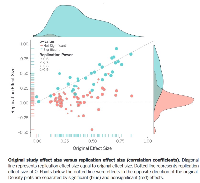
Open Science Collaboration. 2015. “Estimating the Reproducibility of Psychological Science.” Science 349 (6251): aac4716–16. https://doi.org/10.1126/science.aac4716.
Orben, Amy, and Daniel Lakens. 2019. “Crud (Re)defined,” May. https://doi.org/10.31234/osf.io/96dpy.
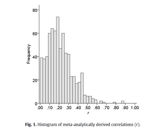
Rains, Stephen A., Timothy R. Levine, and Rene Weber. 2018. “Sixty Years of Quantitative Communication Research Summarized: Lessons from 149 Meta-Analyses.” Annals of the International Communication Association 8985: 1–20. https://doi.org/10.1080/23808985.2018.1446350.
Schäfer, Thomas, and Marcus A. Schwarz. 2019. “The Meaningfulness of Effect Sizes in Psychological Research: Differences Between Sub-Disciplines and the Impact of Potential Biases.” Frontiers in Psychology 10. https://doi.org/10.3389/fpsyg.2019.00813.
Szucs, Denes, and John P. A. Ioannidis. 2017. “Empirical Assessment of Published Effect Sizes and Power in the Recent Cognitive Neuroscience and Psychology Literature.” PLoS Biology 15 (3). https://doi.org/10.1371/journal.pbio.2000797.