    Welch Two Sample t-test

data:  control and treatment
t = -0.58009, df = 194.18, p-value = 0.5625
alternative hypothesis: true difference in means is not equal to 0
95 percent confidence interval:
 -0.3519980  0.1919951
sample estimates:
 mean of x  mean of y
0.03251482 0.11251629
What about two measures from the same person
Think of a typical pre/posttest design
Someone who has a tendency to score low will therefore score low on both pre- and post-test measure
The measures are correlated
We need to take into account that measures come from the same unit when simulating
So how do we get correlated measures?
We need to increase the dimensions
So far, we’ve worked with one dimension: our dependent variable only
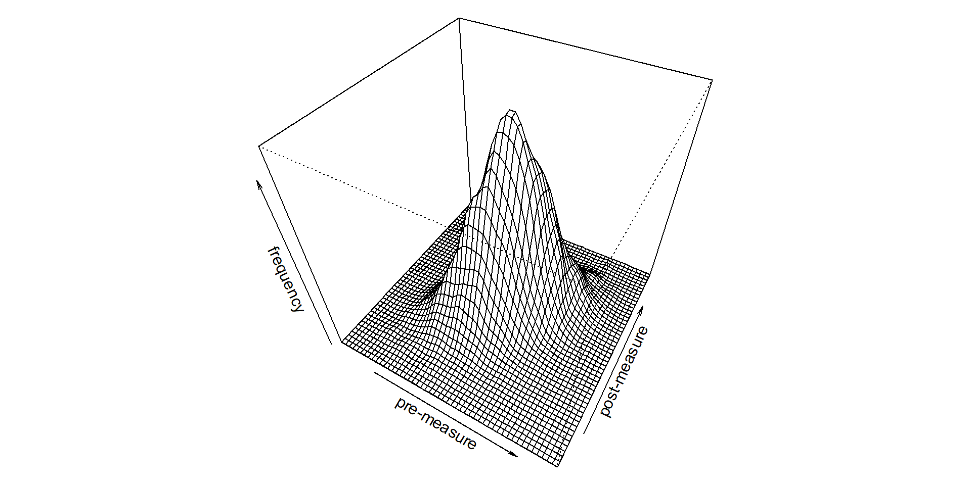
But if a person has multiple measures, that means we don’t just have one normal distribution
We have two correlated normal distributions: a multivariate normal distribution
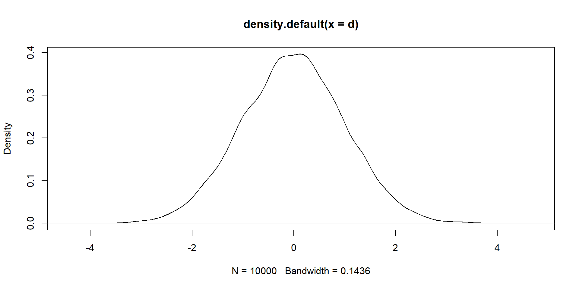
How does that look like?
For univariate, we pick from a single value (left). For bivariate, we pick two values, or a point on the the plane (right).
For the left, we need a mean and SD. What do we need for the right?
What goes into a multivariate distribution
Everything’s double:
2 means
2 SDs
Correlation between variables
An SD for the entire “mountain”
SD = Variance-covariance matrix
The SD for the “mountain” is just the SDs and correlations between the two variables in one place so that we can draw our data from them.
\[
\begin{bmatrix}
var & cov \\
cov & var \\
\end{bmatrix}
\]
This isn’t new
All of you have done correlation tables: they’re just standardized versions of the variance-covariance matrix.
Say we have an experiment where people give us a baseline measure, then the treatment happens, and we get a post-treatment measures. The measures are normally distributed with means of 10 and 10.5 and SDs of 1.5 and 2. The pre- and post-measure are correlated with \(r\) = 0.4.
means <-c(pre =10, post =10.5)pre_sd <-1.5post_sd <-2correlation <-0.4
Getting variance and covariances
SD is just the square root of the variance. So we go \(Var = sd^2\) and we got our variance.
Covariance is just the correlation times the SDs. So we go \(covariance = r(pre, post) \times sd_{pre} \times sd_{post}\)
        pre      post
1  9.750371  7.936974
2 10.001516 10.519466
3 11.279047 10.630203
4 11.081401  8.563613
5 10.086696  9.591592
6 11.432761 10.631188
Let’s check that
Let’s first check the sample to see whether we can recover our numbers.
mean(d$pre); mean(d$post)
[1] 10.00843
[1] 10.48749
sd(d$pre); sd(d$post)
[1] 1.496285
[1] 2.004229
cor(d$pre, d$post)
[1] 0.4119397
Run our test
t.test( d$pre, d$post,paired =TRUE)
    Paired t-test

data:  d$pre and d$post
t = -24.623, df = 9999, p-value < 2.2e-16
alternative hypothesis: true mean difference is not equal to 0
95 percent confidence interval:
 -0.5171917 -0.4409192
sample estimates:
mean difference
     -0.4790554
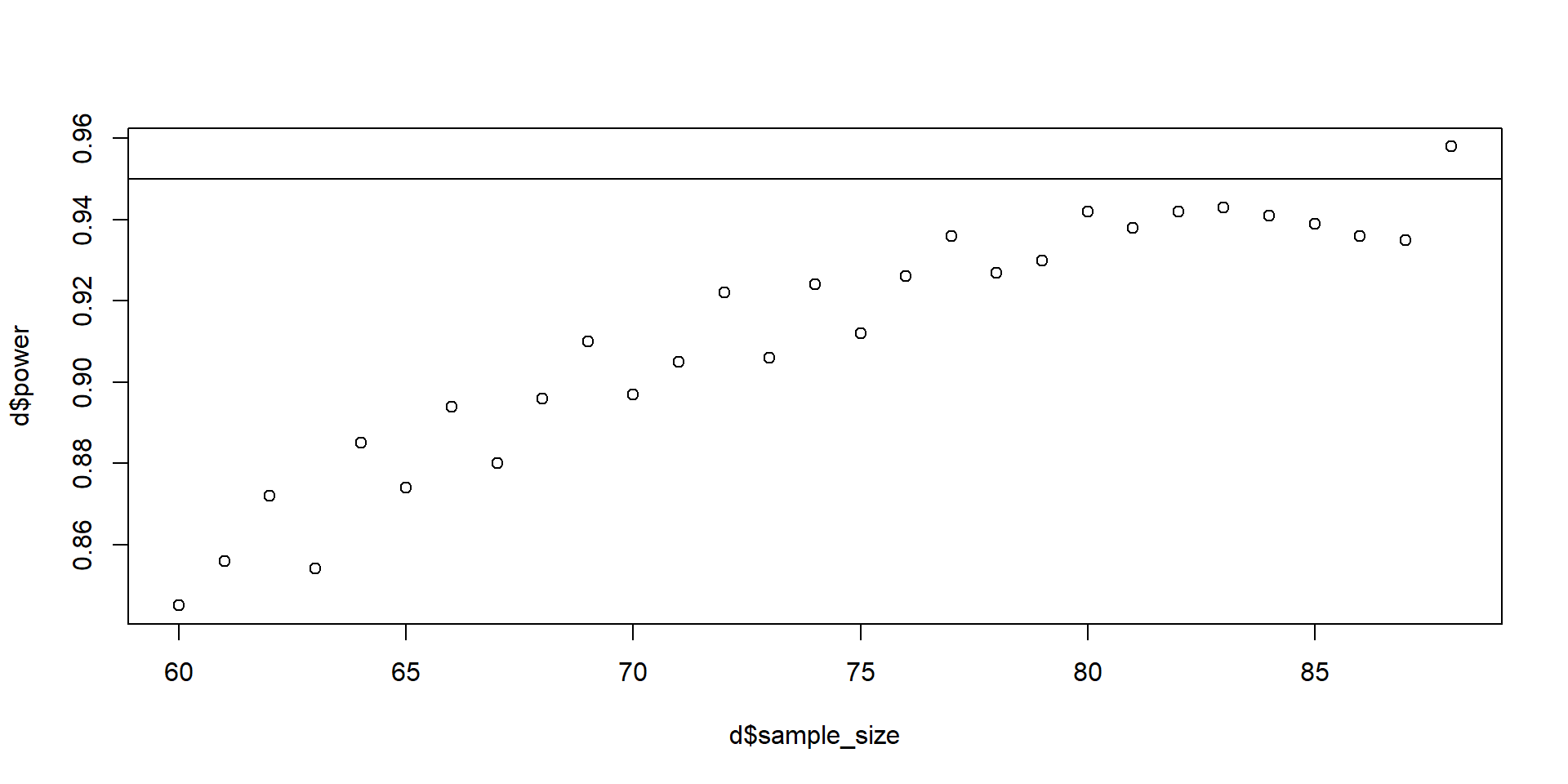
The while operator
Logic
At this point, we’ve worked with for loops and went from a minimum to a maximum. If that maximum is large, that can take quite some time. You can also consider the while function to stop when you’ve reached the point you want to be at.
draws <-1e3n <-60effect_size <-0.5d <-data.frame(sample_size =NULL,power =NULL)power <-0while (power<0.95) { pvalues <-NULLfor (i in1:draws) { control <-rnorm(n) treatment <-rnorm(n, effect_size) t <-t.test(control, treatment, alternative ="less") pvalues[i] <- t$p.value } power <-sum(pvalues<0.05) /length(pvalues) d <-rbind( d,data.frame(sample_size = n,power = power ) ) n <- n +1}