n <- 25
effects <- seq(1, 20, 1)
draws <- 1e3
sd <- 15

outcomes <-
  data.frame(
    effect_size = NULL,
    power = NULL
  )

for (aneffect in effects) {

  pvalues <- NULL

  for (i in 1:draws) {

    control <- rnorm(n, 100, sd)
    treatment <- rnorm(n, 100 + aneffect, sd)
    t <- t.test(control, treatment)

    pvalues[i] <- t$p.value
  }

  outcomes <-
    rbind(
      outcomes,
      data.frame(
        effect_size = aneffect,
        power = sum(pvalues < 0.05) / length(pvalues)
      )
    )
}Alpha, beta, and sensitivity
Power analysis through simulation in R
Niklas Johannes
Takeaways
- Question the default of \(\alpha\) = 0.05 and power = 80%
- Understand how terribly complex designing an informative study is
- Know where to turn when you don’t have enough information
Remember what determines power?
Power is the probability of finding a significant result when there is an effect. It’s determined (simplified) by:
- Effect size
- Sample size
- Error rates (\(\alpha\) and \(\beta\))
The alpha debate
Remember what happens if we change our alpha?
Let’s take a look again.
Remember positive predictive value?
How likely is it that our significant result represents a true effect? Depends on:
- The odds of it being true in the first place (\(R\))
- Our power (how sensitive was our test to detect it)
- Our \(\alpha\) (how many false positives we get)
Reversing the logic
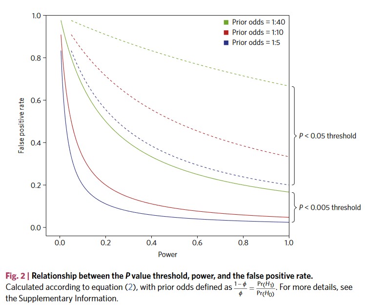
False positive rate: How likely is it that our significant result represents a, well, false positive:
\[\begin{gather*} False \ positive \ rate = \frac{False \ positives}{False \ positives + True \ positives} \end{gather*}\]Formally
- Proportion of null hypotheses that are true (\(\phi\))
- Our error rate for false positives (\(\alpha\))
- Our power (how good are we in finding true positives)
Plug it all in
\[\begin{gather*} False \ positive \ rate = \frac{False \ positives}{False \ positives + True \ positives}\\\\ False \ positives = \phi \times \alpha\\ True \ positives = power \times (1 - \phi)\\\\ False \ positive \ rate = \frac{\phi \times \alpha}{\phi \times \alpha + power \times (1 - \phi)} \end{gather*}\]The \(\alpha\) debate
What’s the effect of alpha?
The \(\alpha\) debate
Counterpoints
- \(\alpha\) = .005 is just as arbitrary
- The biggest factor is still the odds of a hypothesis being true
- We’ll need massive samples = fewer replications and narrower research
Instead: Just like any other thing in our research, we should justify our choice of \(\alpha\).
Why do we even use .05?
Personally, the writer prefers to set a low standard of significance at the 5 per cent point, and ignore entirely all results which fail to reach this level (Fisher 1926).
But right before
If one in twenty does not seem high enough odds, we may, if we prefer it, draw the line at one in fifty or one in a hundred (Fisher 1926).
And why do we use 80% power?
It is proposed here as a convention that, when the investigator has no other basis for setting the desired power value, the value .80 be used. This means that beta is set at .20. This value is offered for several reasons. The chief among them takes into consideration the implicit convention for alpha of .05. The beta of .20 is chosen with the idea that the general relative seriousness of these two kinds of errors is of the order of .20/.05, i.e., that Type I errors are of the order of four times as serious as Type II errors. (Cohen 1988).
Where we stopped reading
This .80 desired power convention is offered with the hope that it will be ignored whenever an investigator can find a basis in his substantive concerns in his specific research investigation to choose a value ad hoc errors. (Cohen 1988).
Unethical?
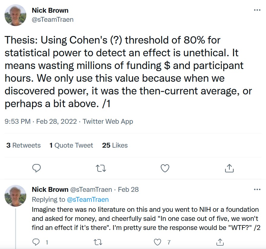
The tyranny of rules of thumb
We might naively assume that when all researchers do something, there must be a good reason for such an established practice. An important step towards maturity as a scholar is the realization that this is not the case. [Maier and Lakens (2021), p. 4]
Should we just replace one rule of thumb with another rule of thumb?
That Koala example
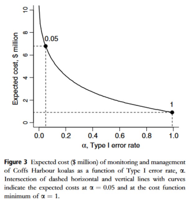
Better safe than sorry?
Imagine you’re thirsty. You down a glass of milk. Right after drinking it, you think that it tasted funny.
- H1: The milk was expired.
- H0: The milk wasn’t expired.
How should we act?
Expired milk means a night of diarrhea. Imagine there’s a pill that will prevent that, with no side effects. How should you act?
- Type I error: You act as if the milk was expired even though it wasn’t (false positive).
- Type II error: You act as if the milk wasn’t expired even though it was (false negative).
Assessing the consequences
Consequences:
- Type I error: None.
- Type II error: Severe.
We should always act as if H1 is true: \(\alpha\) = 1.
A statistical reason
Remember this?

Jeffreys-Lindley’s paradox
With great power…
- Large samples (or massive effects) result in extremely high power (e.g., 99%)
- Remember Crud: Anything could be significant
- We should consider lowering the \(\alpha\)
Balancing and minimizing
- They’re called errors for a reasons
- They have a costs, so we want to reduce them
- Leads to effective decision making
They’re not independent
- \(\alpha\) influences our power
- Power is \((1 - \beta)\) (e.g., when power 87%, then our \(\beta\) = .13)
- Change \(\alpha\), change \(\beta\)
A worked example
Let’s assume we’re comparing two groups. We’re certain the effect exists (Cohen’s \(d\) = 0.5) because there’s lots of literature. We decide to go with the conventional thresholds for our error rates (although we should know better). Therefore:
- \(\alpha\) = .05
- \(\beta\) = .20 (aka power is 80%)
- Prior odds of H1 being true: 3:1
What’s our (real) Type I error rate?
Probability of committing a false positive: How many nulls are there and what’s our chance of falsely flagging a null as a true effect?
\[\begin{gather*} Probability \ H_0 \ is \ true \times Probability \ Type \ I \ error \\ P(H_0) \times \alpha \end{gather*}\]What’s our (real) Type II error rate?
Probability of commmiting a false negative: How many true effects are there and what’s our chance of missing them?
\[\begin{gather*} Probability \ H_1 \ is \ true \times Probability \ Type \ II \ error \\ P(H_1) \times \beta \end{gather*}\]Weighted combined error rate
Let’s combine our (real) Type I and Type II error rates and put them in:
- \(\alpha\) = .05
- \(\beta\) = .20 (aka power is 80%)
- Prior odds of H1 being true: 3:1 (i.e., 75%)
Is that the best we can do?
Now let’s change our \(\alpha\) to 0.10. That makes our power go up to 88%. Our \(\beta\), therefore, is .12. (Remember: iterative). Put those in:
\[\begin{gather*} (P(H_0) \times \alpha) + (P(H_1) \times \beta) \\ (0.25 \times 0.10) + (0.75 \times 0.12) = 0.115 \end{gather*}\]Comparing the two
Raising the alpha, in this case, decreases our combined error rate. What’s the optimum?
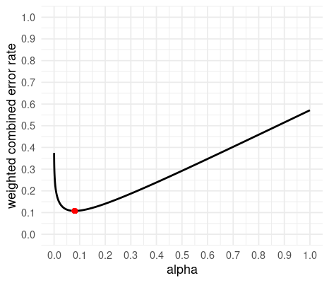
Try it out.
Pesky reality
What if the probabilities of our hypotheses are different? Say the odds of H1 being true aren’t 3:1, but 1:3.
\[\begin{gather*} (0.75 \times 0.05) + (0.25 \times 0.20) = 0.0875\\ (0.75 \times 0.10) + (0.25 \times 0.12) = 0.105 \end{gather*}\]Try it out.
General logic
If an effect is likely, we don’t want to miss it. We cast a wider net and consider more effects significant because the (real) risk of false positives is lowered. The higher \(P(H_1)\), the less strict \(\alpha\).
If an effect is unlikely, we don’t want to falsely claim it’s there. We cast a narrower net and consider less effects significant because the (real) risk of false positive is increased. The higher \(P(H_0)\), the more strict \(\alpha\).
A balancing act
- Ideally, we balance prior probabilities and cost-benefits
- Prior probabilities influence expected number of errors
- But we must still weigh the relative costs of these errors
Remember the milk?
When \(P(H_0)\) is high and we don’t lower our alpha, we have a completely unbalanced error rate with a super high false positive rate. Whenever we drink funny tasting milk, we’ll make the error and assume it has expired (and therefore take the pill). The low costs of Type I errors justifies making lots of them, but not making Type II errors.
Try it out.
Some considerations
- Publishing a false positive: bad!
- But the benefits could be huge: publish away then!
- But it costs a lot to get these benefits: Hm, maybe not.
The compromise
When we know the effect size, the sample size, and what ratio of \(\alpha\) and \(\beta\) we want, we’re performing a compromise analysis. It finds the optimum point of high power and the right ratio. It’s usually performed with very small or very large samples.
Lots of moving parts
What if we don’t know our sample size?
- SESOI
- Costs of Type I and Type II errors
- Prior probabilities
- What we want the combined error rate to be
Try it out.
The Bible
Other ways
- Measure entire population
- Resource constraints
- Accuracy
- A priori power analysis
- Heuristics
- No justification
Resource constraints
- Sometimes we have limited resources
- Need to balance our resources over the course of a project
- Is it worth conducting the study?
Is it worth it?
Depends on our goal.
- If we have to make a decision: Any data will be helpful and a compromise analysis is a good idea
- If we’re interested in the effect: Will a meta-analysis be performed?
- Then consider a sensitivity analysis
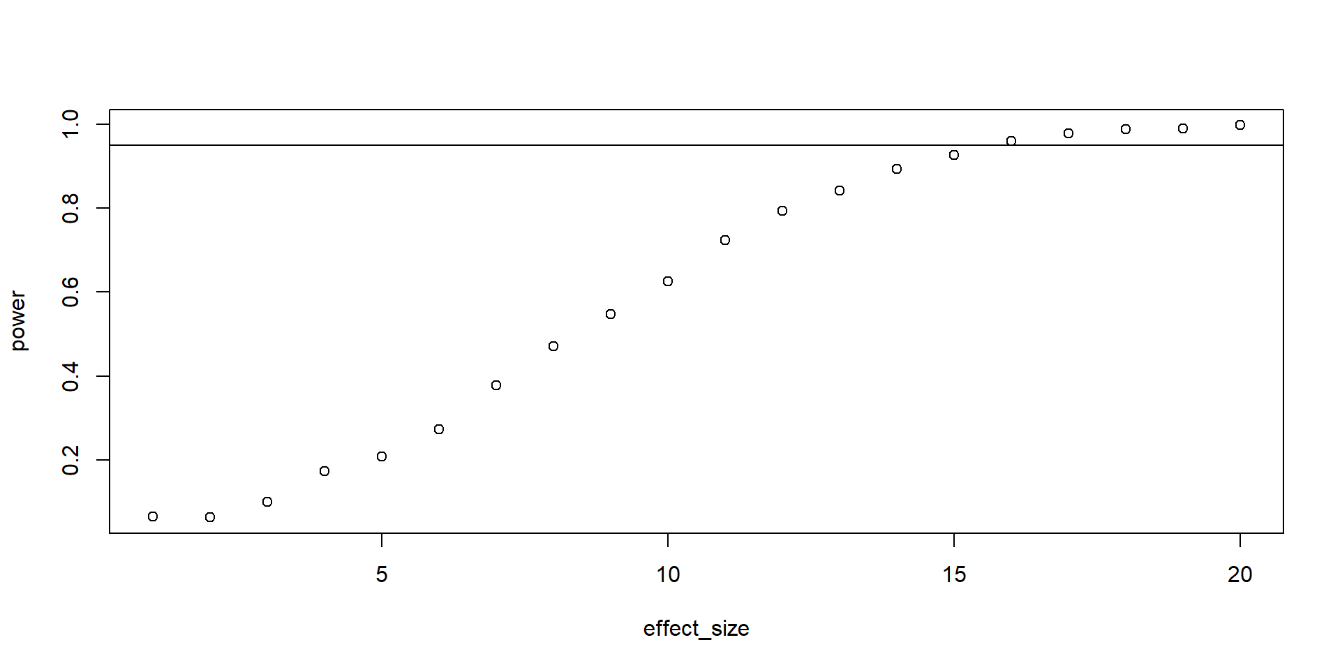
Sensitivity analysis
Reverses the logic:
- If we have a given sample size (aka what our resources allow to collect)
- Which effect size can we detect with how much power given our sample size?
- Compare that effect to your SESOI
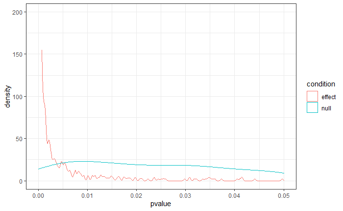
Simulating sensitivity
Plotting
Takeaways
- Question the default of \(\alpha\) = 0.05 and power = 80%
- Understand how terribly complex designing an informative study is
- Know where to turn when you don’t have enough information
Let’s get simulating
References
Benjamin, Daniel J., James O. Berger, Magnus Johannesson, Brian A. Nosek, E.-J. Wagenmakers, Richard Berk, Kenneth A. Bollen, et al. 2018. “Redefine Statistical Significance.” Nature Human Behaviour 2 (1): 6–10. https://doi.org/10.1038/s41562-017-0189-z.
Cohen, J. 1988. Statistical Power Analysis for the Behavioral Sciences. 2nd ed. Hillsdale, NJ: Lawrence Erlbaum.
Field, Scott A., Andrew J. Tyre, Niclas Jonzen, Jonathan R. Rhodes, and Hugh P. Possingham. 2004. “Minimizing the Cost of Environmental Management Decisions by Optimizing Statistical Thresholds.” Ecology Letters 7 (8): 669–75. https://doi.org/10.1111/j.1461-0248.2004.00625.x.
Fisher, Ronald A. 1926. “The Arrangement of Field Experiments.” Journal of the Ministry of Agriculture 33: 503–15.
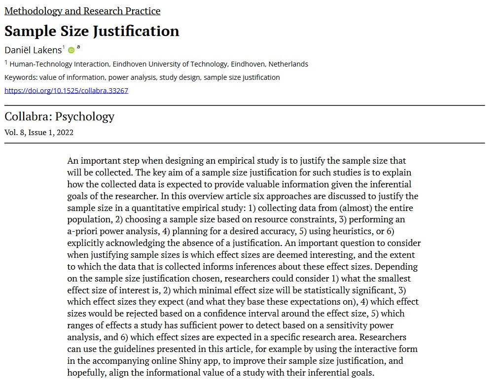
Lakens, Daniël. 2022. “Sample Size Justification.” Collabra: Psychology 8 (1): 33267. https://doi.org/10.1525/collabra.33267.
Lakens, Daniël, Federico G. Adolfi, Casper J. Albers, Farid Anvari, Matthew A. J. Apps, Shlomo E. Argamon, Thom Baguley, et al. 2018. “Justify Your Alpha.” Nature Human Behaviour 2 (3): 168–71. https://doi.org/10.1038/s41562-018-0311-x.
Maier, Maximilian, and Daniel Lakens. 2021. “Justify Your Alpha: A Primer on Two Practical Approaches,” June. https://doi.org/10.31234/osf.io/ts4r6.