The linear model and comparing multiple groups

Power analysis through simulation in R

Niklas Johannes

Takeaways

Understand the logic behind the data generating process
See how the linear model is our data generating process
Apply this to a setting with multiple categories in a predictor

Lots of foreshadowing

Data generating process
Simulations are that process

What’s that data generating process?

The process, in the real world, that you believe created the data
We don’t know the process, but we can observe the outcomes
When we try to explain the outcome, we make assumptions about the data generating process
We collect data from samples and want to know whether our assumptions fit (and generalize)

What’s the process?

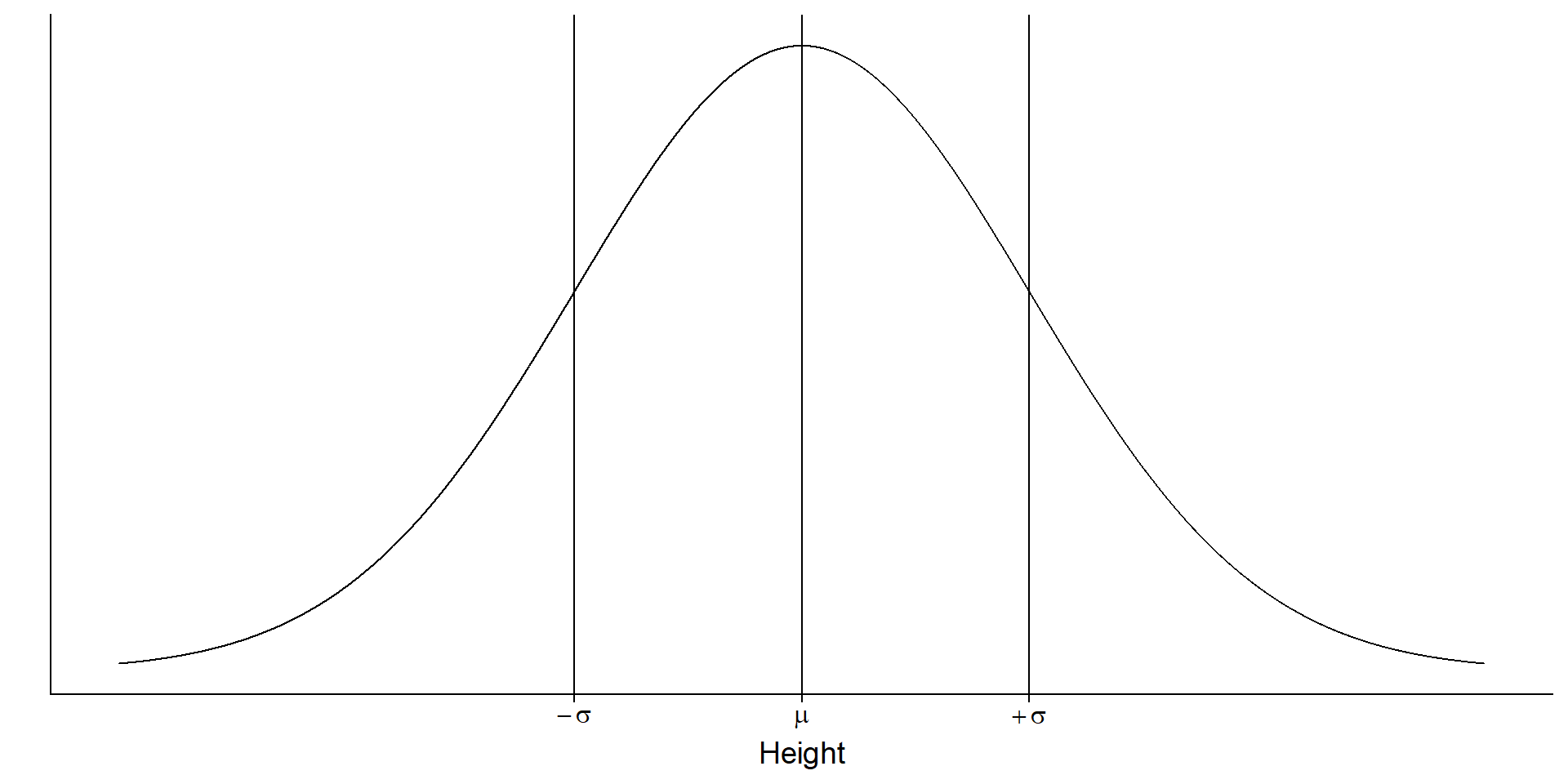
You measure height in a sample (the observable consequences). What’s the data generating process?

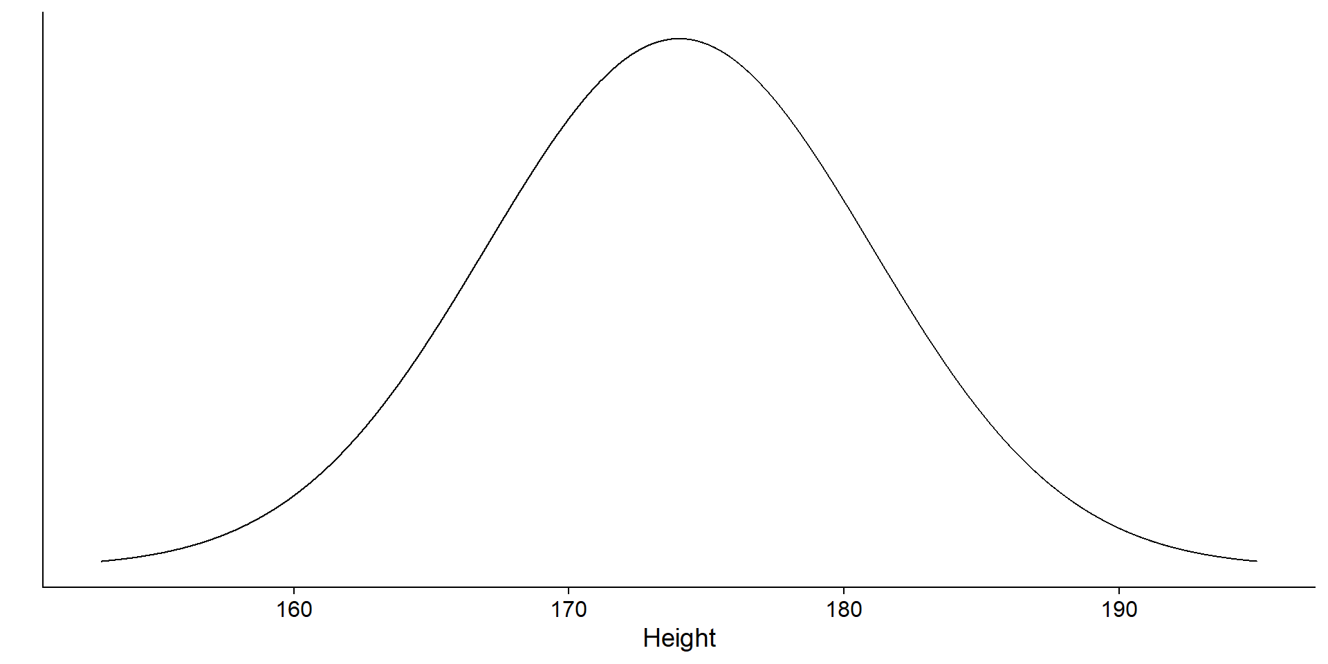
We have a (simple) process

\(Normal(\mu, \sigma)\)

Look familiar?

\(Normal(174, 7)\) aka rnorm(174, 7)

plot(density(rnorm(1e4, 174, 7)))

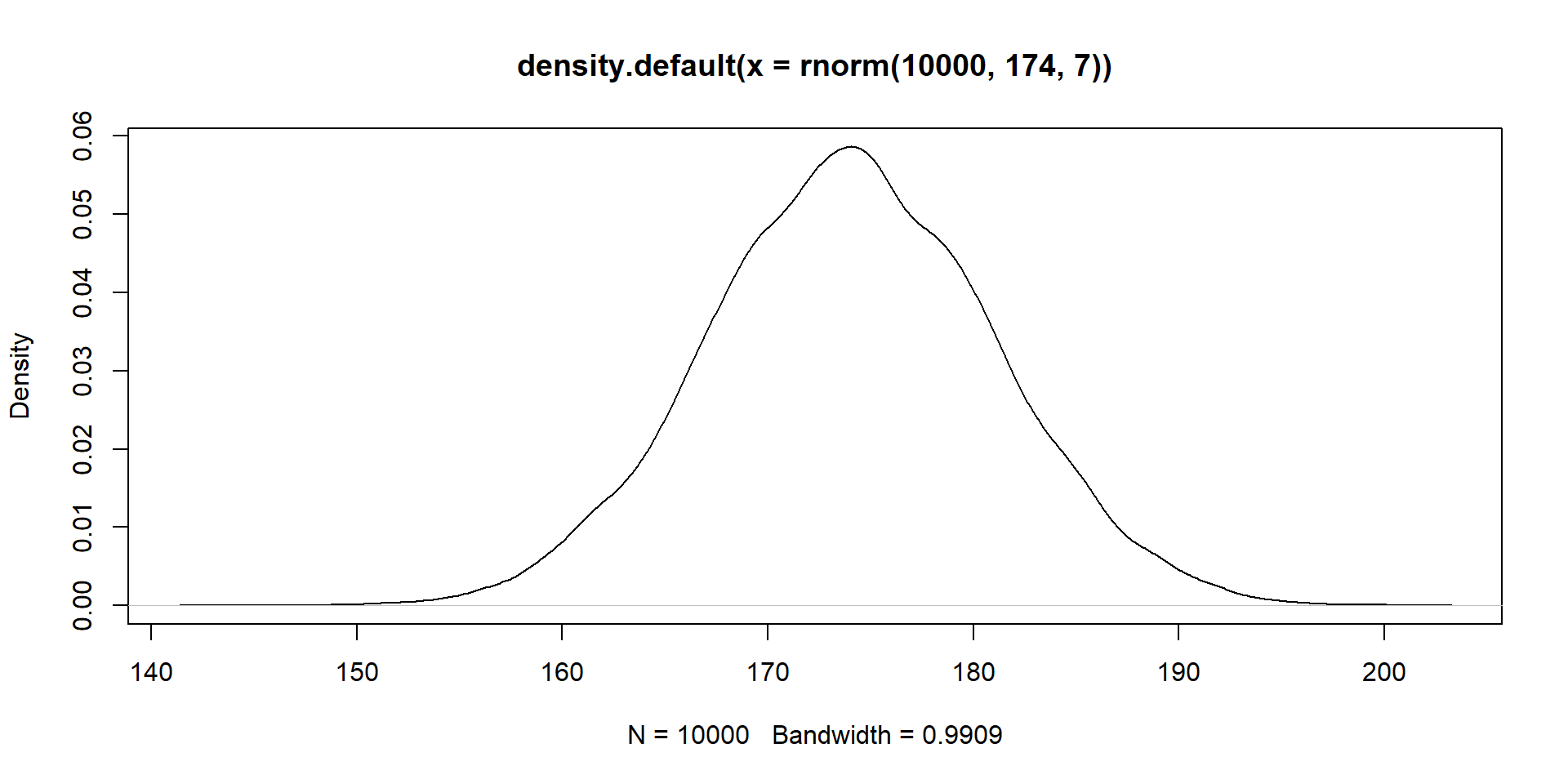
All are processes

rnorm: You say that the underlying data generating process is a normal distribution
rbinom: You say that the underlying data generating process is a binomial distribution
You get the idea

Important: Those are assumptions you make explicit and they can be wrong.

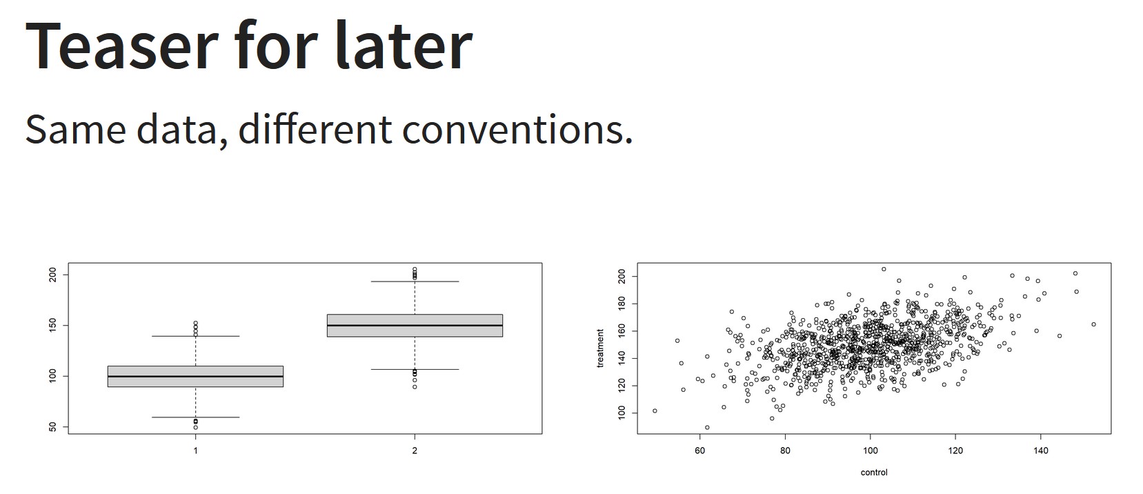
Remember our t-tests?

You are explicitly claiming that the observable outcome (the data) have been generated by this true underlying process. The process is a normal distribution with a true effect size (\(\mu\)) and a true standard deviation (\(\sigma\)) for two data generating processes: \(Normal(100, 15)\) and \(Normal(105, 15)\)

control <- rnorm(100, 100, 15)
treatment <- rnorm(100, 105, 15)

t.test(control, treatment)


    Welch Two Sample t-test

data:  control and treatment
t = -0.57372, df = 197.92, p-value = 0.5668
alternative hypothesis: true difference in means is not equal to 0
95 percent confidence interval:
 -5.495395  3.018476
sample estimates:
mean of x mean of y 
 100.3389  101.5774

That’s why simulation is cool

You’re being explicit about your model of the world
You translate that model (data generating process) into a concrete formula (code) to create data (the consequences of the data generation process)
You check how changes to your model influence the data, which inform the conclusions you draw from the data about your model (aka statistical inference)
No more hiding your model assumptions behind standard software

This all sounds complicated

Here’s the good news: In (much of) the (social) sciences we rely on a common data generating process: the linear model.

t-test, regression, logistic regression, machine learning are all variations of the linear model.

\(y = \beta_0 + \beta_1x\)

All stolen from here

Source

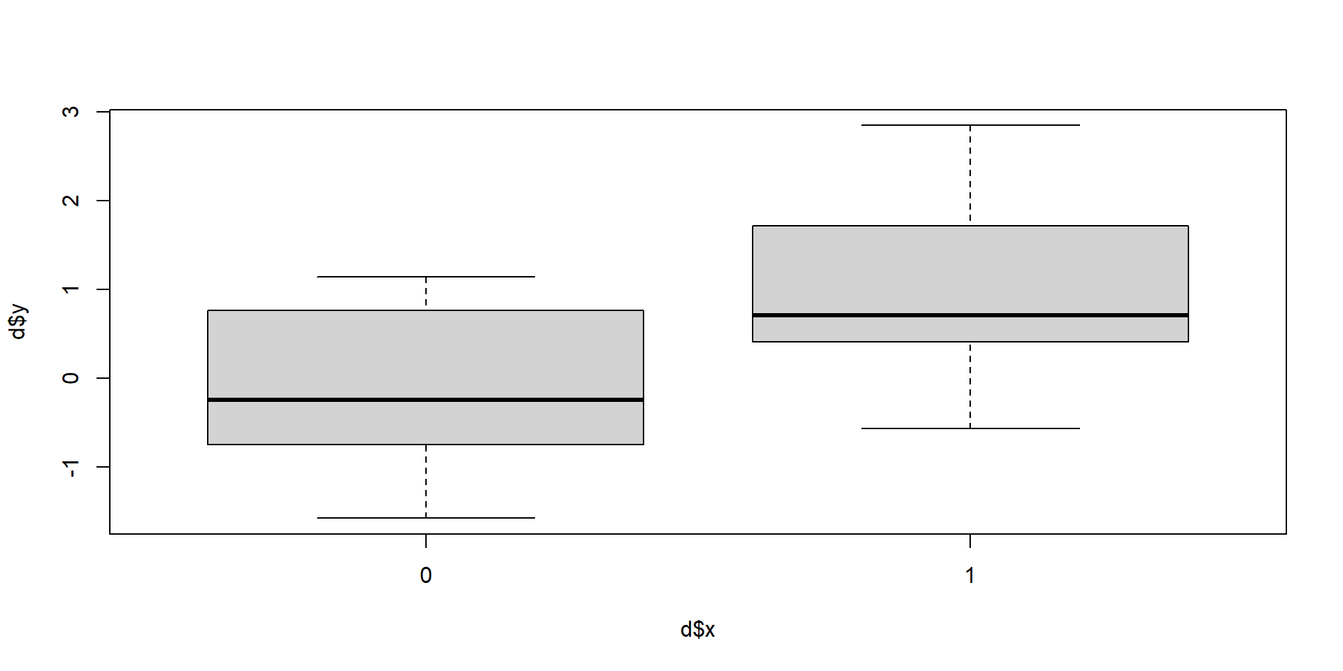
Back to our control and treatment

\(y = \beta_0 + \beta_1x\): What’s \(x\) here?

control <- rnorm(15, 0, 1)
treatment <- rnorm(15, 1, 1)

Group membership

Our group is \(x\).

d <- 
  data.frame(
    group = rep(c("control", "treatment"), each = 15),
    y = c(control, treatment)
  )

d$x <- ifelse(d$group=="control", 0, 1)

group	y	x
control	-0.2462229	0
control	-0.9597997	0
control	-0.5238199	0
control	1.1407442	0
control	-0.6588351	0
control	-1.5772346	0
control	0.6479015	0
control	-0.1497161	0
control	1.0852342	0
control	0.4002139	0
control	0.9653700	0
control	0.8700338	0
control	-0.8435252	0
control	-1.4519022	0
control	-0.4569357	0
treatment	2.4476205	1
treatment	0.2285001	1
treatment	0.8593449	1
treatment	1.2349919	1
treatment	-0.1423595	1
treatment	0.5735239	1
treatment	0.7055050	1
treatment	2.4935786	1
treatment	-0.5713438	1
treatment	0.4377587	1
treatment	2.8445324	1
treatment	1.7562574	1
treatment	0.5085672	1
treatment	0.3798965	1
treatment	1.6759042	1

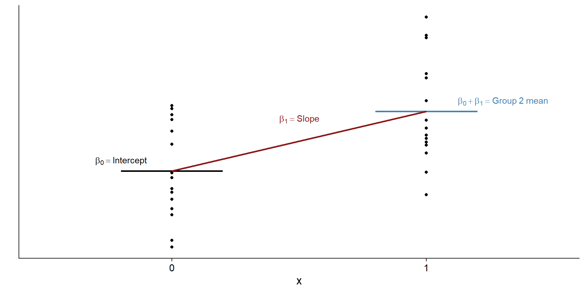
What happens when \(x\) is zero?

\[\begin{align} & y = \beta_0 + \beta_1x\\ & y = \beta_0 + \beta_1 \times 0\\ & y = \beta_0 \end{align}\]

In other words, when we predict values for the control (aka \(x=0\)) group, our best predictor for outcome scores becomes \(\beta_0\) (also known as the intercept): the mean for the control group.

What happens when \(x\) is one?

\[\begin{align} & y = \beta_0 + \beta_1x\\ & y = \beta_0 + \beta_1 \times 1\\ & y = \beta_0 + \beta_1\\ & y = mean(control) + ? \end{align}\]

We already know that the intercept (\(\beta_0\)) is the mean of the control group. How would we now go from that mean to predicting scores of the treatment group? What do we need to add to the mean of the control group to get the mean of the treatment group?

Pictures, please

Let’s check that

Mean of the control group (our intercept or \(\beta_0\)):

mean(d$y[d$x==0])

[1] -0.1172329

Difference (our slope or \(\beta_1\)):

mean(d$y[d$x==1]) - mean(d$y[d$x==0])

[1] 1.146051

Mean of the treatment group (\(\beta_0 + \beta_1\)):

mean(d$y[d$x==1])

[1] 1.028819

Linear model:

model <- lm(y ~ x, data = d)

summary(model)


Call:
lm(formula = y ~ x, data = d)

Residuals:
    Min      1Q  Median      3Q     Max 
-1.6002 -0.6345 -0.2464  0.7557  1.8157 

Coefficients:
            Estimate Std. Error t value Pr(>|t|)   
(Intercept)  -0.1172     0.2496  -0.470  0.64225   
x1            1.1461     0.3530   3.246  0.00303 **
---
Signif. codes:  0 '***' 0.001 '**' 0.01 '*' 0.05 '.' 0.1 ' ' 1

Residual standard error: 0.9668 on 28 degrees of freedom
Multiple R-squared:  0.2735,    Adjusted R-squared:  0.2475 
F-statistic: 10.54 on 1 and 28 DF,  p-value: 0.003027

So they’re really the same?

t.test(control, treatment, var.equal = TRUE)


    Two Sample t-test

data:  control and treatment
t = -3.2464, df = 28, p-value = 0.003027
alternative hypothesis: true difference in means is not equal to 0
95 percent confidence interval:
 -1.8691755 -0.4229274
sample estimates:
 mean of x  mean of y 
-0.1172329  1.0288185

summary(lm(y ~ x, d))


Call:
lm(formula = y ~ x, data = d)

Residuals:
    Min      1Q  Median      3Q     Max 
-1.6002 -0.6345 -0.2464  0.7557  1.8157 

Coefficients:
            Estimate Std. Error t value Pr(>|t|)   
(Intercept)  -0.1172     0.2496  -0.470  0.64225   
x1            1.1461     0.3530   3.246  0.00303 **
---
Signif. codes:  0 '***' 0.001 '**' 0.01 '*' 0.05 '.' 0.1 ' ' 1

Residual standard error: 0.9668 on 28 degrees of freedom
Multiple R-squared:  0.2735,    Adjusted R-squared:  0.2475 
F-statistic: 10.54 on 1 and 28 DF,  p-value: 0.003027

Same logic for a one-sample t-test

There’s no \(x\) here, so all we’re left with is the intercept, which we test against our H₀. A single number (aka the mean) predicts \(y\).

\[\begin{align} & y = \beta_0 \end{align}\]

Pictures, please

Let’s check that once more

Mean of the treatment group (our intercept or \(\beta_0\)):

mean(d$y[d$x==1])

[1] 1.028819

Linear model:

model <- lm(y ~ 1, data = d[d$x==1,])

summary(model)


Call:
lm(formula = y ~ 1, data = d[d$x == 1, ])

Residuals:
    Min      1Q  Median      3Q     Max 
-1.6002 -0.6200 -0.3233  0.6873  1.8157 

Coefficients:
            Estimate Std. Error t value Pr(>|t|)   
(Intercept)   1.0288     0.2619   3.929  0.00151 **
---
Signif. codes:  0 '***' 0.001 '**' 0.01 '*' 0.05 '.' 0.1 ' ' 1

Residual standard error: 1.014 on 14 degrees of freedom

So they’re really the same?

t.test(treatment)


    One Sample t-test

data:  treatment
t = 3.9289, df = 14, p-value = 0.001513
alternative hypothesis: true mean is not equal to 0
95 percent confidence interval:
 0.467180 1.590457
sample estimates:
mean of x 
 1.028819

summary(lm(y ~ 1, d[d$x==1,]))


Call:
lm(formula = y ~ 1, data = d[d$x == 1, ])

Residuals:
    Min      1Q  Median      3Q     Max 
-1.6002 -0.6200 -0.3233  0.6873  1.8157 

Coefficients:
            Estimate Std. Error t value Pr(>|t|)   
(Intercept)   1.0288     0.2619   3.929  0.00151 **
---
Signif. codes:  0 '***' 0.001 '**' 0.01 '*' 0.05 '.' 0.1 ' ' 1

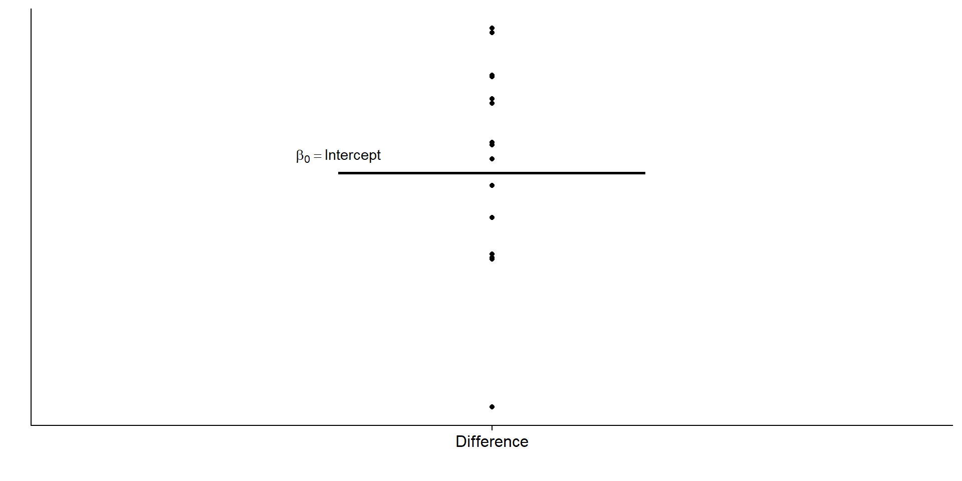
Residual standard error: 1.014 on 14 degrees of freedom

Same logic for a paired-samples t-test

Remember: Paired samples t-test is just testing the difference in scores against H₀. This way, it turns into a one-sample t-test, so all we’re left with is, once again, the intercept, which we test against our H₀. A single number (aka the mean) predicts \(y\) (technically \(y_{difference}\)).

\[\begin{align} & y_{treatment} - y_{control} = \beta_0 \end{align}\]

Pictures, please

Let’s check that once more

Mean of the difference (our intercept or \(\beta_0\)):

mean(treatment-control)

[1] 1.146051

Linear model:

model <- lm(treatment-control ~ 1)

summary(model)


Call:
lm(formula = treatment - control ~ 1)

Residuals:
    Min      1Q  Median      3Q     Max 
-2.8026 -0.8407  0.2060  0.8599  1.5478 

Coefficients:
            Estimate Std. Error t value Pr(>|t|)   
(Intercept)   1.1461     0.3052   3.754  0.00213 **
---
Signif. codes:  0 '***' 0.001 '**' 0.01 '*' 0.05 '.' 0.1 ' ' 1

Residual standard error: 1.182 on 14 degrees of freedom

So they’re really the same?

t.test(treatment-control)


    One Sample t-test

data:  treatment - control
t = 3.7545, df = 14, p-value = 0.002134
alternative hypothesis: true mean is not equal to 0
95 percent confidence interval:
 0.4913576 1.8007453
sample estimates:
mean of x 
 1.146051

summary(lm(treatment-control ~ 1))


Call:
lm(formula = treatment - control ~ 1)

Residuals:
    Min      1Q  Median      3Q     Max 
-2.8026 -0.8407  0.2060  0.8599  1.5478 

Coefficients:
            Estimate Std. Error t value Pr(>|t|)   
(Intercept)   1.1461     0.3052   3.754  0.00213 **
---
Signif. codes:  0 '***' 0.001 '**' 0.01 '*' 0.05 '.' 0.1 ' ' 1

Residual standard error: 1.182 on 14 degrees of freedom

What about ANOVA then?

Same as before: We predict scores with the group membership (aka the mean in each group). Doesn’t matter whether we predict it from two (t-test) or more groups (ANOVA). Now we just have an indicator for membership for each group: dummy coding.

groups	\(x_1\)	\(x_2\)
control	0	0
low	1	0
high	0	1

\[\begin{align} & y = \beta_0 + \beta_1x_1 + \beta_2x_2 \end{align}\]

Getting the score for control

groups	\(x_1\)	\(x_2\)
control	0	0
low	1	0
high	0	1

\[\begin{align} & y = \beta_0 + \beta_1x_1 + \beta_2x_2\\ & y = \beta_0 + \beta_1 \times 0 + \beta_2 \times 0\\ & y = \beta_0 \end{align}\]

Getting the score for low

groups	\(x_1\)	\(x_2\)
control	0	0
low	1	0
high	0	1

\[\begin{align} & y = \beta_0 + \beta_1x_1 + \beta_2x_2\\ & y = \beta_0 + \beta_1 \times 1 + \beta_2 \times 0\\ & y = \beta_0 + \beta_1 \end{align}\]

Getting the score for high

groups	\(x_1\)	\(x_2\)
control	0	0
low	1	0
high	0	1

\[\begin{align} & y = \beta_0 + \beta_1x_1 + \beta_2x_2\\ & y = \beta_0 + \beta_1 \times 0 + \beta_2 \times 1\\ & y = \beta_0 + \beta_2 \end{align}\]

What are \(\beta_1\) and \(\beta_2\) then?

What do we need to go from the control mean to the low mean? What do we need to go from control mean to high mean? Same as with the t-test: the difference between those means.

Pictures, please

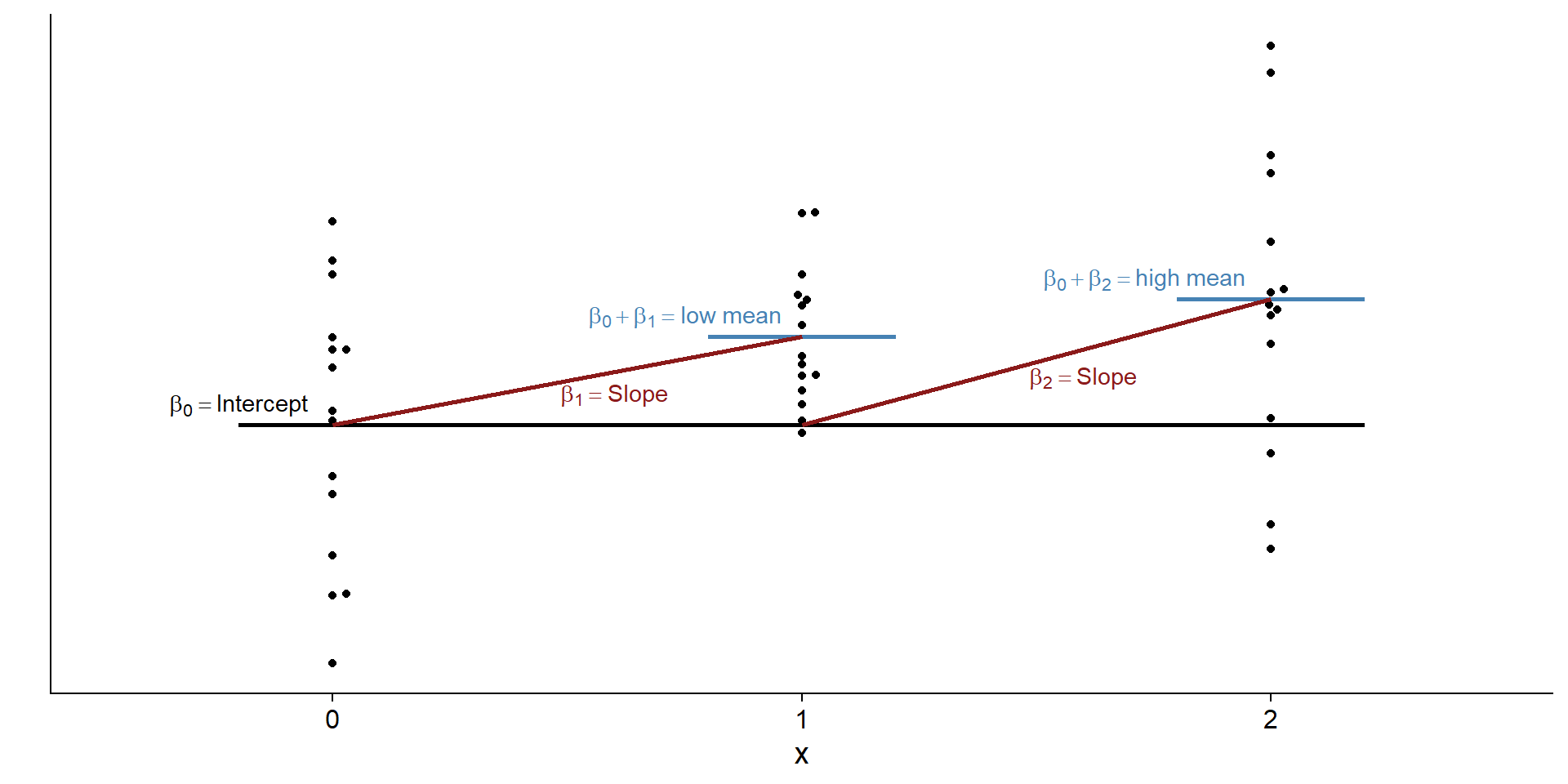
Just an extension

If we know how to simulate a t-test, we know how to simulate an ANOVA (because both are just linear models): Imitate the data generating process.

\[\begin{align} & y = \beta_0 + \beta_1x_1 + \beta_2x_2 \end{align}\]

n <- 5

control <- rnorm(n, 100, 15)
low <- rnorm(n, 120, 15)
high <- rnorm(n, 140, 15)

d <- data.frame(
  y = c(control, low, high),
  condition = rep(c("control", "low", "high"), each = n)
)

d$condition <- as.factor(d$condition)

Add our dummy codes

d$group_low <- rep(c(0, 1, 0), each = n)
d$group_high <- rep(c(0, 0, 1), each = n)

           y condition group_low group_high
1  106.49227   control         0          0
2   87.82910   control         0          0
3  121.66152   control         0          0
4   93.52831   control         0          0
5  109.83472   control         0          0
6  124.82888       low         1          0
7  108.24242       low         1          0
8  143.63591       low         1          0
9  129.64349       low         1          0
10 121.34641       low         1          0
11 144.14826      high         0          1
12 150.18933      high         0          1
13 141.34749      high         0          1
14  95.10365      high         0          1
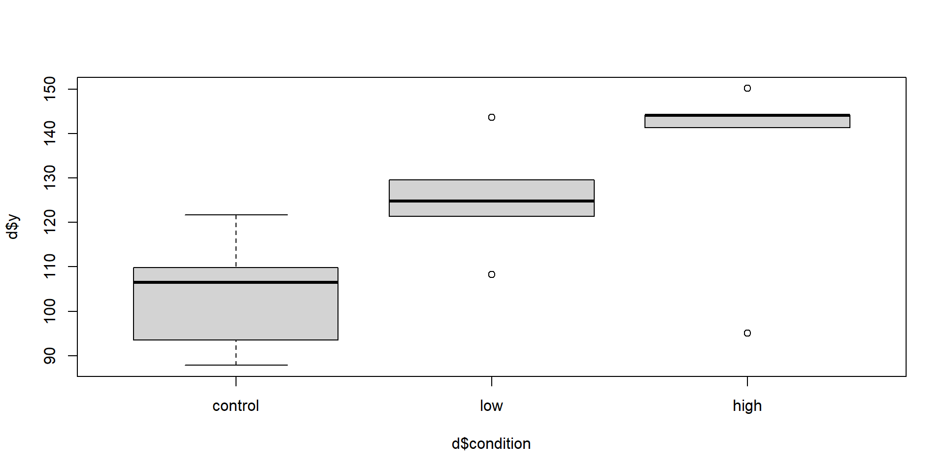
15 144.27324      high         0          1

Compare to model

# A tibble: 3 × 2
  condition  mean
  <fct>     <dbl>
1 control    104.
2 low        126.
3 high       135.

model <- lm(y ~ group_low + group_high, data = d)

summary(model)


Call:
lm(formula = y ~ group_low + group_high, data = d)

Residuals:
    Min      1Q  Median      3Q     Max 
-39.909  -7.267   4.104   9.198  18.096 

Coefficients:
            Estimate Std. Error t value Pr(>|t|)    
(Intercept)  103.869      7.547  13.763 1.04e-08 ***
group_low     21.670     10.673   2.030   0.0651 .  
group_high    31.143     10.673   2.918   0.0129 *  
---
Signif. codes:  0 '***' 0.001 '**' 0.01 '*' 0.05 '.' 0.1 ' ' 1

Residual standard error: 16.88 on 12 degrees of freedom
Multiple R-squared:  0.4272,    Adjusted R-squared:  0.3317 
F-statistic: 4.475 on 2 and 12 DF,  p-value: 0.03532

Compare to ANOVA

our_anova <- aov(y ~ condition, data = d)

summary(our_anova)

            Df Sum Sq Mean Sq F value Pr(>F)  
condition    2   2549  1274.4   4.475 0.0353 *
Residuals   12   3417   284.8                 
---
Signif. codes:  0 '***' 0.001 '**' 0.01 '*' 0.05 '.' 0.1 ' ' 1

our_regression <- lm(y ~ group_low + group_high, data = d)

summary(our_regression)


Call:
lm(formula = y ~ group_low + group_high, data = d)

Residuals:
    Min      1Q  Median      3Q     Max 
-39.909  -7.267   4.104   9.198  18.096 

Coefficients:
            Estimate Std. Error t value Pr(>|t|)    
(Intercept)  103.869      7.547  13.763 1.04e-08 ***
group_low     21.670     10.673   2.030   0.0651 .  
group_high    31.143     10.673   2.918   0.0129 *  
---
Signif. codes:  0 '***' 0.001 '**' 0.01 '*' 0.05 '.' 0.1 ' ' 1

Residual standard error: 16.88 on 12 degrees of freedom
Multiple R-squared:  0.4272,    Adjusted R-squared:  0.3317 
F-statistic: 4.475 on 2 and 12 DF,  p-value: 0.03532

No need to use dummies

The lm call will automatically dummy code factors.

summary(lm(y ~ condition, data = d))


Call:
lm(formula = y ~ condition, data = d)

Residuals:
    Min      1Q  Median      3Q     Max 
-39.909  -7.267   4.104   9.198  18.096 

Coefficients:
              Estimate Std. Error t value Pr(>|t|)    
(Intercept)    103.869      7.547  13.763 1.04e-08 ***
conditionhigh   31.143     10.673   2.918   0.0129 *  
conditionlow    21.670     10.673   2.030   0.0651 .  
---
Signif. codes:  0 '***' 0.001 '**' 0.01 '*' 0.05 '.' 0.1 ' ' 1

Residual standard error: 16.88 on 12 degrees of freedom
Multiple R-squared:  0.4272,    Adjusted R-squared:  0.3317 
F-statistic: 4.475 on 2 and 12 DF,  p-value: 0.03532

In a power simulation

n <- 40
m1 <- 100
m2 <- 103
m3 <- 105
sd <- 8
draws <- 1e4

pvalues <- NULL

for (i in 1:n) {

  group1 <- rnorm(n, m1, sd)
  group2 <- rnorm(n, m2, sd)
  group3 <- rnorm(n, m3, sd)

  dat <- data.frame(
    scores = c(group1, group2, group3),
    condition = as.factor(rep(c("group1", "group2", "group3"), each = n))
  )

  m <- summary(lm(scores ~ condition, data = dat))
  
  pvalues[i] <- broom::glance(m)$p.value
}

sum(pvalues < 0.05) / length(pvalues)

[1] 0.7

Getting that p-value

You can access the p-value by storing the summary in an object (as a list) and accessing its component. For the lm summary, that’s a bit less straightforward. See https://stackoverflow.com/questions/5587676/pull-out-p-values-and-r-squared-from-a-linear-regression.

About that effect size

Let’s just swap the low and high conditions.

d2 <- d

levels(d2$condition) <- c("control", "low", "high")

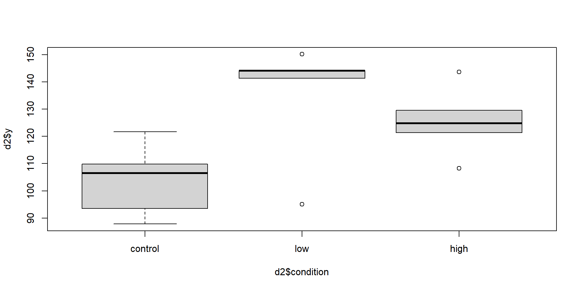
Now what are the model statistics?

summary(lm(y ~ condition, d))


Call:
lm(formula = y ~ condition, data = d)

Residuals:
    Min      1Q  Median      3Q     Max 
-39.909  -7.267   4.104   9.198  18.096 

Coefficients:
              Estimate Std. Error t value Pr(>|t|)    
(Intercept)    103.869      7.547  13.763 1.04e-08 ***
conditionlow    21.670     10.673   2.030   0.0651 .  
conditionhigh   31.143     10.673   2.918   0.0129 *  
---
Signif. codes:  0 '***' 0.001 '**' 0.01 '*' 0.05 '.' 0.1 ' ' 1

Residual standard error: 16.88 on 12 degrees of freedom
Multiple R-squared:  0.4272,    Adjusted R-squared:  0.3317 
F-statistic: 4.475 on 2 and 12 DF,  p-value: 0.03532

summary(lm(y ~ condition, d2))


Call:
lm(formula = y ~ condition, data = d2)

Residuals:
    Min      1Q  Median      3Q     Max 
-39.909  -7.267   4.104   9.198  18.096 

Coefficients:
              Estimate Std. Error t value Pr(>|t|)    
(Intercept)    103.869      7.547  13.763 1.04e-08 ***
conditionlow    31.143     10.673   2.918   0.0129 *  
conditionhigh   21.670     10.673   2.030   0.0651 .  
---
Signif. codes:  0 '***' 0.001 '**' 0.01 '*' 0.05 '.' 0.1 ' ' 1

Residual standard error: 16.88 on 12 degrees of freedom
Multiple R-squared:  0.4272,    Adjusted R-squared:  0.3317 
F-statistic: 4.475 on 2 and 12 DF,  p-value: 0.03532

What about the effect size?

effectsize::eta_squared(lm(y ~ condition, d))

# Effect Size for ANOVA

Parameter | Eta2 |       95% CI
-------------------------------
condition | 0.43 | [0.03, 1.00]

- One-sided CIs: upper bound fixed at [1.00].

effectsize::eta_squared(lm(y ~ condition, d2))

# Effect Size for ANOVA

Parameter | Eta2 |       95% CI
-------------------------------
condition | 0.43 | [0.03, 1.00]

- One-sided CIs: upper bound fixed at [1.00].

How would I go for power now?

Back to standardized vs. unstandardized
Best to “draw” first
Determine contrast of interest

What about correlated measures?

Remember drawing two scores from the same unit?

\[ \begin{bmatrix} var & cov \\ cov & var \\ \end{bmatrix} \]

We just need to extend that to the number of measures:

\[ \begin{bmatrix} var & cov & cov\\ cov & var & cov\\ cov & cov & var \end{bmatrix} \]

What we need to know

The standard deviation for each measure (\(\sigma_{x_1}\))
The correlation between each measure (\(r_{x_1x_2}\))

\[ \begin{bmatrix} SD_{x_1} & r_{x_1x_2} & r_{x_1x_3}\\ r_{x_2x_1} & SD_{x_2} & r_{x_2x_3}\\ r_{x_3x_1} & r_{x_3x_2} & SD_{x_3} \end{bmatrix} \]

Same as before

Define our parameters and get variance-covariance matrix.

means <- c(control = 100, low = 103, high = 105)
sd <- 8
correlation <- 0.4
covariance <- correlation * sd * sd

our_matrix <- matrix(
  c(
    sd**2, covariance, covariance,
    covariance, sd**2, covariance,
    covariance, covariance, sd**2
  ),
  ncol = 3
)

our_matrix

     [,1] [,2] [,3]
[1,] 64.0 25.6 25.6
[2,] 25.6 64.0 25.6
[3,] 25.6 25.6 64.0

Then draw from multivariate normal

library(MASS)

set.seed(42)

d <- 
  mvrnorm(
    200,
    means,
    our_matrix
  )
d <- as.data.frame(d)
d$id <- factor(1:200)
head(d)

    control       low      high id
1 102.65124  93.16169  86.70051  1
2  98.88458 109.62849 109.98486  2
3  94.79098  97.77544 108.68290  3
4  90.66920  94.06642 111.49926  4
5  98.78622 106.29663  95.40168  5
6  99.54111 110.82243  99.60934  6

Let’s check

Can we recover our numbers of means = c(100, 103, 105), SD of 8, and correlation of 0.4?

mean(d$control); mean(d$low); mean(d$high)

[1] 99.89351

[1] 103.4035

[1] 105.214

sd(d$control); sd(d$low); sd(d$high)

[1] 7.854443

[1] 7.706208

[1] 8.024822

cor(d$control, d$low); cor(d$control, d$high); cor(d$low, d$high);

[1] 0.3166429

[1] 0.4616155

[1] 0.3740047

We can’t use `lm` this time

The linear model has several assumptions, one of which is that observations are independent. They clearly aren’t (we specified a correlation between them after all). So we need to go for models that take this dependence into account.

For most cases, data need to be in the long format:

library(tidyr)

d2 <- 
  pivot_longer(
    d,
    cols = -id,
    names_to = "condition",
    values_to = "score"
  )

Long format

control	low	high	id
102.65124	93.16169	86.70051	1
98.88458	109.62849	109.98486	2
94.79098	97.77544	108.68290	3
90.66920	94.06642	111.49926	4
98.78622	106.29663	95.40168	5
99.54111	110.82243	99.60934	6

id	condition	score
1	control	102.65124
1	low	93.16169
1	high	86.70051
2	control	98.88458
2	low	109.62849
2	high	109.98486

Let’s run the RM ANOVA

model <- aov(score ~ condition + Error(id), d2)
summary(model)


Error: id
           Df Sum Sq Mean Sq F value Pr(>F)
Residuals 199  21774   109.4               

Error: Within
           Df Sum Sq Mean Sq F value   Pr(>F)    
condition   2   2927    1464   38.48 5.25e-16 ***
Residuals 398  15135      38                     
---
Signif. codes:  0 '***' 0.001 '**' 0.01 '*' 0.05 '.' 0.1 ' ' 1

Just a (hierarchical) linear model

summary(model)


Error: id
           Df Sum Sq Mean Sq F value Pr(>F)
Residuals 199  21774   109.4               

Error: Within
           Df Sum Sq Mean Sq F value   Pr(>F)    
condition   2   2927    1464   38.48 5.25e-16 ***
Residuals 398  15135      38                     
---
Signif. codes:  0 '***' 0.001 '**' 0.01 '*' 0.05 '.' 0.1 ' ' 1

library(lme4)

model2 <- lmer(score ~ condition + (1 | id), d2)
anova(model2)

Analysis of Variance Table
          npar Sum Sq Mean Sq F value
condition    2   2927  1463.5  38.484

Check here for more background info.

This is the max

The workshop won’t go further than (interactions) with repeated measures. More resources on simulating more complicated designs at the final wrap up.

Takeaways

Understand the logic behind the data generating process
See how the linear model is our data generating process
Apply this to a setting with multiple categories in a predictor

The linear model and comparing multiple groups

Takeaways

Lots of foreshadowing

What’s that data generating process?

What’s the process?

We have a (simple) process

Look familiar?

All are processes

Remember our t-tests?

That’s why simulation is cool

This all sounds complicated

All stolen from here

Back to our control and treatment

Group membership

Finding our inputs again

What happens when \(x\) is zero?

What happens when \(x\) is one?

Pictures, please

Let’s check that

So they’re really the same?

Same logic for a one-sample t-test

Pictures, please

Let’s check that once more

So they’re really the same?

Same logic for a paired-samples t-test

Pictures, please

Pictures, please

Let’s check that once more

So they’re really the same?

What about ANOVA then?

Getting the score for control

Getting the score for low

Getting the score for high

What are \(\beta_1\) and \(\beta_2\) then?

Pictures, please

Just an extension

Add our dummy codes

Compare to model

Compare to ANOVA

No need to use dummies

In a power simulation

Getting that p-value

About that effect size

Now what are the model statistics?

What about the effect size?

How would I go for power now?

What about correlated measures?

What we need to know

Same as before

Then draw from multivariate normal

Let’s check

We can’t use lm this time

Long format

Let’s run the RM ANOVA

Just a (hierarchical) linear model

This is the max

Takeaways

Let’s get simulating

We can’t use `lm` this time