Interactions

Power analysis through simulation in R

Niklas Johannes

Takeaways

• Understand what an interaction is from the perspective of the linear model
• Make yourself think in more detail about the form of interactions
• Be able to translate that detail to generating data

What’s an interaction?

• Tells us whether the effect of one variable depends on another variable
• Extension of the linear model
• In effect, it just checks whether lines are parallel

Is there an interaction?

How about now?

And now?

Definitely now

What’s the interaction then?

• In all of these models, we need to ask what extra information about the outcome being in both groups gives us beyond individual group membership
• If the line isn’t parallel, combined group membership gives us additional info than just individual group membership
• When we simulate, that’s our data generating process: The info each group membership carries as well as their combination

Back to the linear model

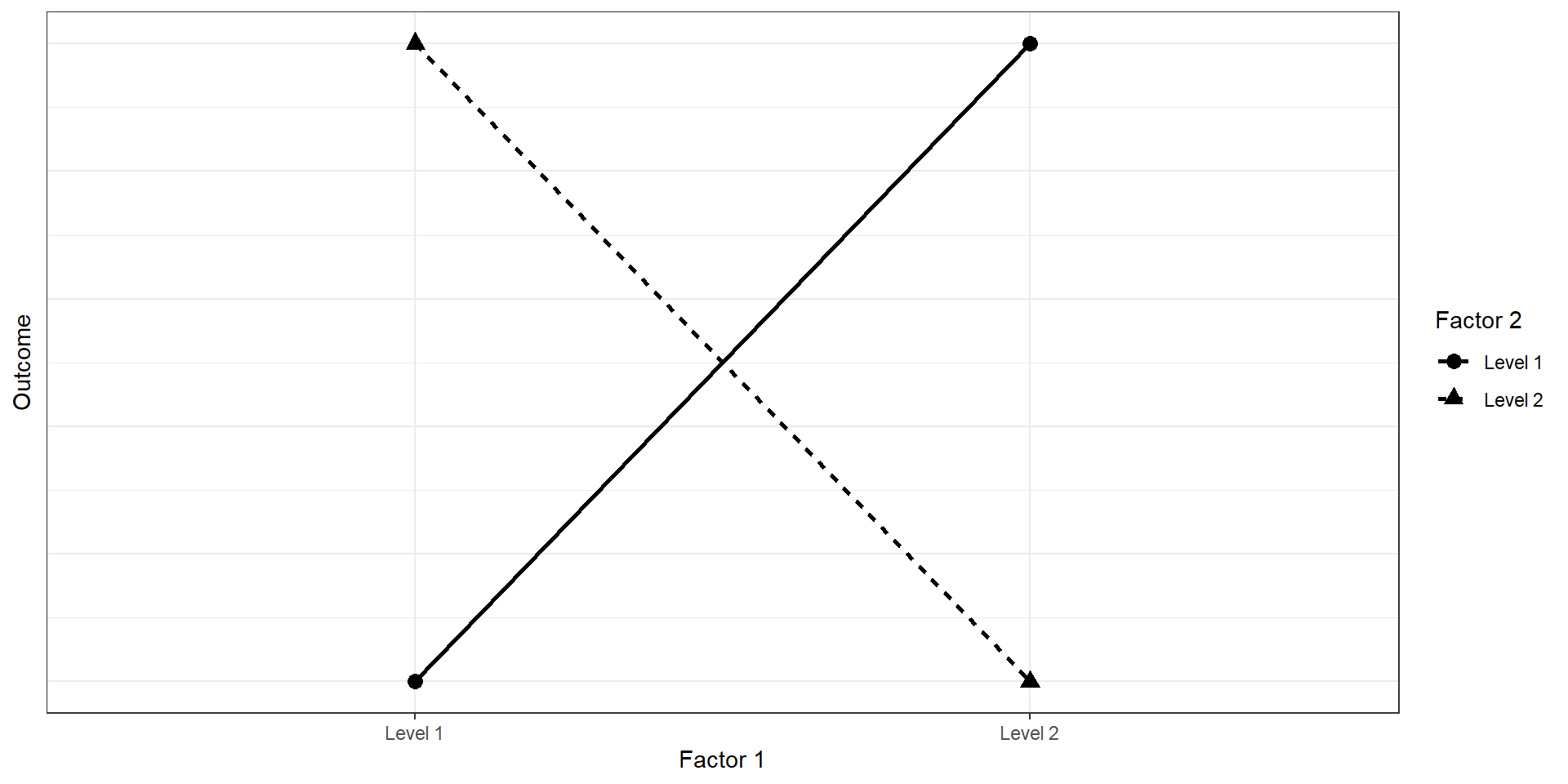
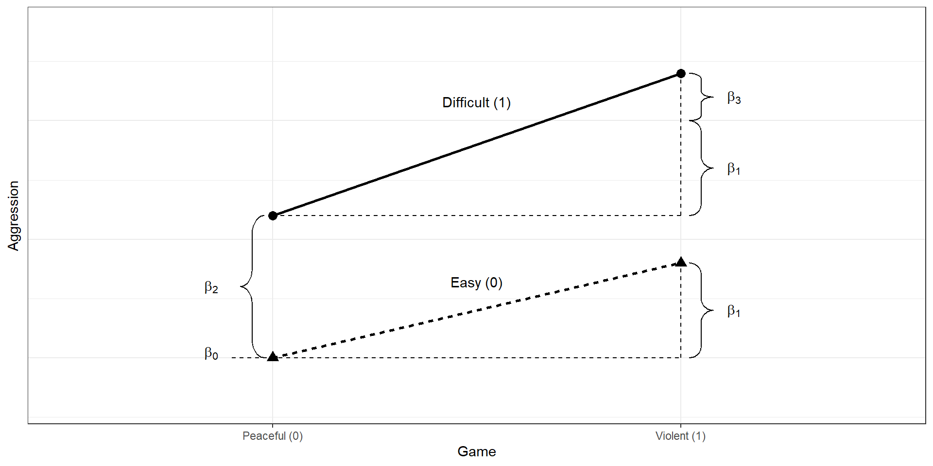
Say we want to see the effect of playing a violent game on feelings of aggression, but suspect the effect depends on the difficulty of the game. We have 2 factors with 2 levels each:

• Game: Peaceful vs. Violent
• Difficulty: Easy vs. Hard

Both as dummies

We code both as dummies:

Game	Difficulty	x1	x2
Peaceful	Easy	0	0
Violent	Easy	1	0
Peaceful	Hard	0	1
Violent	Hard	1	1

In our linear model

\[ Aggression = \beta_0 + \beta_1Game + \beta_2Difficulty + \beta_3Game \times Difficulty \]

Let’s go through

Game	Difficulty	x1	x2
Peaceful	Easy	0	0
Violent	Easy	1	0
Peaceful	Hard	0	1
Violent	Hard	1	1

\[\begin{align} & Aggression = \beta_0 + \beta_1Game + \beta_2Difficulty + \beta_3Game \times Difficulty\\ & Aggression = \beta_0 + \beta_1 \times 0 + \beta_2 \times 0 + \beta_3 \times 0 \times 0\\ & Aggression = \beta_0 \end{align}\]

Pictures, please

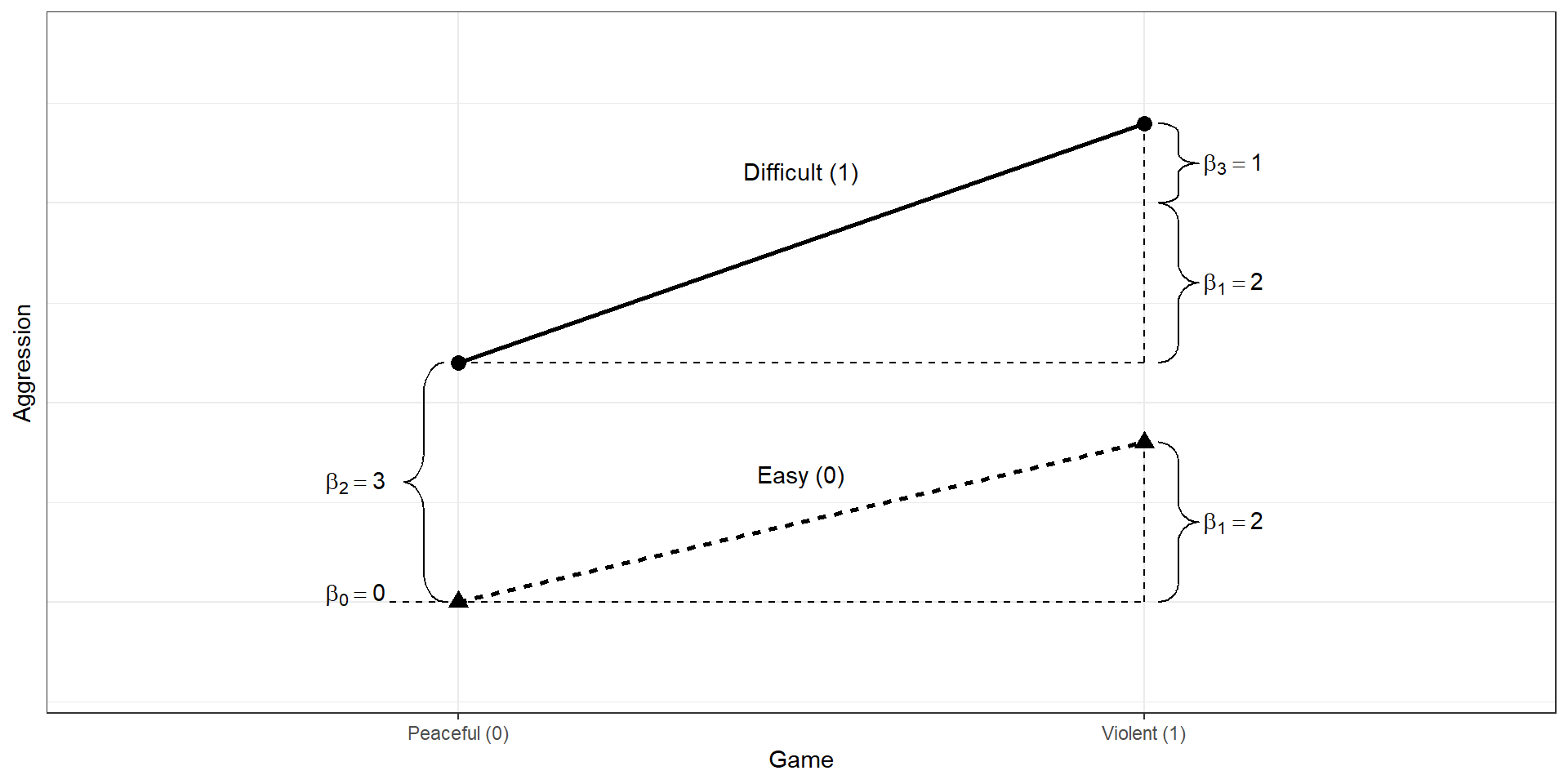
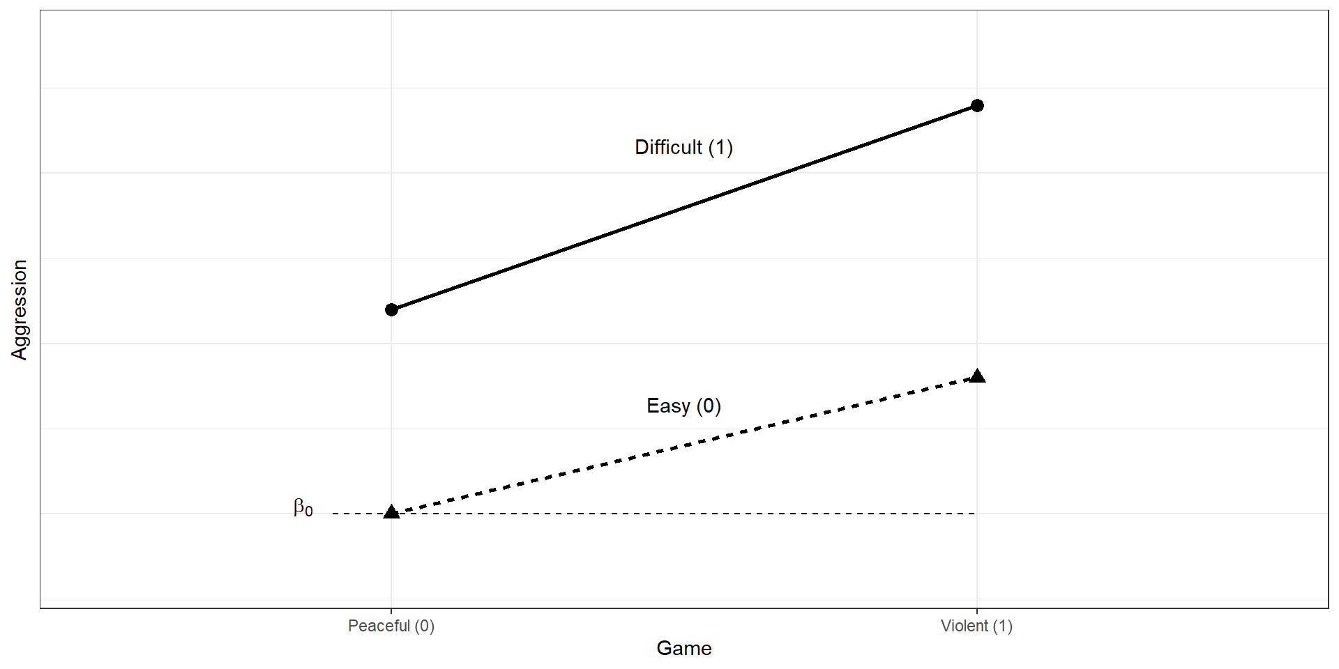
\(\beta_0\) is the mean of a peaceful and easy game.

Let’s go through

Game	Difficulty	x1	x2
Peaceful	Easy	0	0
Violent	Easy	1	0
Peaceful	Hard	0	1
Violent	Hard	1	1

\[\begin{align} & Aggression = \beta_0 + \beta_1Game + \beta_2Difficulty + \beta_3Game \times Difficulty\\ & Aggression = \beta_0 + \beta_1 \times 1 + \beta_2 \times 0 + \beta_3 \times 1 \times 0\\ & Aggression = \beta_0 + \beta_1 \end{align}\]

Pictures, please

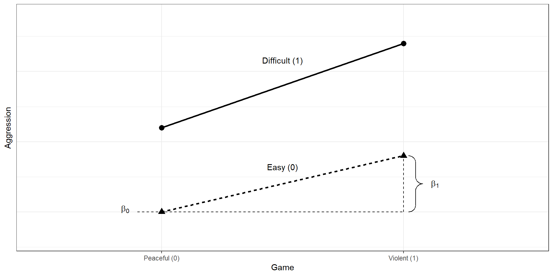
\(\beta_1\) is the difference between a peaceful and a violent game for easy games.

Let’s go through

Game	Difficulty	x1	x2
Peaceful	Easy	0	0
Violent	Easy	1	0
Peaceful	Hard	0	1
Violent	Hard	1	1

\[\begin{align} & Aggression = \beta_0 + \beta_1Game + \beta_2Difficulty + \beta_3Game \times Difficulty\\ & Aggression = \beta_0 + \beta_1 \times 0 + \beta_2 \times 1 + \beta_3 \times 0 \times 1\\ & Aggression = \beta_0 + \beta_2 \end{align}\]

Pictures, please

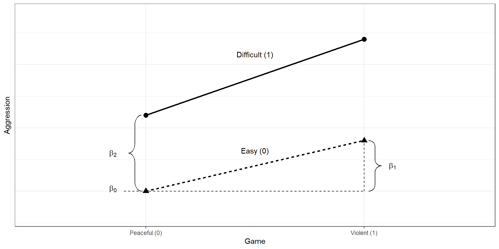
\(\beta_2\) is the difference between an easy and a difficult game for peaceful games.

Let’s go through

Game	Difficulty	x1	x2
Peaceful	Easy	0	0
Violent	Easy	1	0
Peaceful	Hard	0	1
Violent	Hard	1	1

\[\begin{align} & Aggression = \beta_0 + \beta_1Game + \beta_2Difficulty + \beta_3Game \times Difficulty\\ & Aggression = \beta_0 + \beta_1 \times 1 + \beta_2 \times 1 + \beta_3 \times 1 \times 1\\ & Aggression = \beta_0 + \beta_2 + \beta_3 \end{align}\]

Pictures, please

\(\beta_3\) is the extra difference between a peaceful and violent game when the game is also difficult.

Let’s put that into numbers

Let’s say we have 50 people per group.

d <- 
  data.frame(
    Game = rep(0:1, times = 50*2),
    Difficulty = rep(0:1, each = 50*2)
  )

table(d$Game, d$Difficulty)

   
     0  1
  0 50 50
  1 50 50

Let’s put that into numbers

Then we imitate our regression equation (and add some error):

\(Aggression = \beta_0 + \beta_1Game + \beta_2Difficulty + \beta_3Game \times Difficulty\)

b0 <- 0 # peaceful and easy
b1 <- 2 # difference between b0 and violent and easy
b2 <- 3 # difference between b0 and peaceful and hard
b3 <- 1 # the "extra"

set.seed(42)

d$Aggression <- 
  b0 + b1*d$Game + b2*d$Difficulty + b3*d$Game*d$Difficulty + rnorm(200, 0, 1)

Where are our values?

b0 <- 0 # peaceful and easy
b1 <- 2 # difference between b0 and violent and easy
b2 <- 3 # difference between b0 and peaceful and hard
b3 <- 1 # the "extra"

Let’s recover our values

summary(lm(Aggression ~ Game*Difficulty, d))

Call:
lm(formula = Aggression ~ Game * Difficulty, data = d)

Residuals:
     Min       1Q   Median       3Q      Max 
-3.02981 -0.58291  0.04749  0.61717  2.72220 

Coefficients:
                Estimate Std. Error t value Pr(>|t|)    
(Intercept)      0.03672    0.13845   0.265    0.791    
Game             1.99159    0.19579  10.172  < 2e-16 ***
Difficulty       2.80863    0.19579  14.345  < 2e-16 ***
Game:Difficulty  1.14275    0.27689   4.127 5.43e-05 ***
---
Signif. codes:  0 '***' 0.001 '**' 0.01 '*' 0.05 '.' 0.1 ' ' 1

Residual standard error: 0.979 on 196 degrees of freedom
Multiple R-squared:  0.8298,    Adjusted R-squared:  0.8272 
F-statistic: 318.6 on 3 and 196 DF,  p-value: < 2.2e-16

Might as well go for means?

Game	Difficulty	Betas	Values	Means
Peaceful	Easy	\(\beta_0\)	0	0
Violent	Easy	\(\beta_0+\beta_1\)	0+2	2
Peaceful	Hard	\(\beta_0+\beta_2\)	0+3	3
Violent	Hard	\(\beta_0+\beta_1+\beta_2+\beta_3\)	0+2+3+1	6

Directly make the groups

set.seed(42)

peace_easy <- 0
violent_easy <- 2
peace_hard <- 3
violent_hard <- 6

d <- 
  data.frame(
    Game = rep(c(0, 1), each = 50, times = 2),
    Difficulty = rep(c(0, 1), each = 50*2),
    Aggression = c(
      rnorm(50, peace_easy, 1),
      rnorm(50, violent_easy, 1),
      rnorm(50, peace_hard, 1),
      rnorm(50, violent_hard, 1)
    )
  )

Same result

summary(lm(Aggression ~ Game*Difficulty, d))

Call:
lm(formula = Aggression ~ Game * Difficulty, data = d)

Residuals:
     Min       1Q   Median       3Q      Max 
-3.09379 -0.57416  0.02313  0.58649  2.85314 

Coefficients:
                Estimate Std. Error t value Pr(>|t|)    
(Intercept)     -0.03567    0.13829  -0.258 0.796720    
Game             2.13637    0.19557  10.924  < 2e-16 ***
Difficulty       2.88442    0.19557  14.748  < 2e-16 ***
Game:Difficulty  0.99116    0.27658   3.584 0.000428 ***
---
Signif. codes:  0 '***' 0.001 '**' 0.01 '*' 0.05 '.' 0.1 ' ' 1

Residual standard error: 0.9779 on 196 degrees of freedom
Multiple R-squared:  0.8323,    Adjusted R-squared:  0.8297 
F-statistic: 324.1 on 3 and 196 DF,  p-value: < 2.2e-16

A more extreme example

peace_easy <- 0
violent_easy <- 3
peace_hard <- 3
violent_hard <- 0

d <- 
  data.frame(
    Game = rep(c(0, 1), each = 50, times = 2),
    Difficulty = rep(c(0, 1), each = 50*2),
    Aggression = c(
      rnorm(50, peace_easy, 1),
      rnorm(50, violent_easy, 1),
      rnorm(50, peace_hard, 1),
      rnorm(50, violent_hard, 1)
    )
  )

Full cross-over

What’s our “correction”?

summary(lm(Aggression ~ Game*Difficulty, d))

Call:
lm(formula = Aggression ~ Game * Difficulty, data = d)

Residuals:
     Min       1Q   Median       3Q      Max 
-2.67125 -0.66907 -0.00832  0.65231  2.48827 

Coefficients:
                Estimate Std. Error t value Pr(>|t|)    
(Intercept)      0.00794    0.13457   0.059    0.953    
Game             2.96338    0.19031  15.571   <2e-16 ***
Difficulty       2.93052    0.19031  15.398   <2e-16 ***
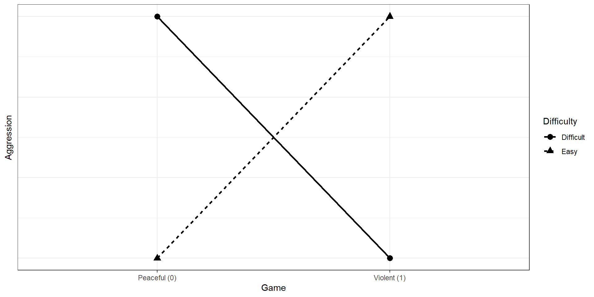
Game:Difficulty -5.77443    0.26915 -21.455   <2e-16 ***
---
Signif. codes:  0 '***' 0.001 '**' 0.01 '*' 0.05 '.' 0.1 ' ' 1

Residual standard error: 0.9516 on 196 degrees of freedom
Multiple R-squared:  0.7016,    Adjusted R-squared:  0.697 
F-statistic: 153.6 on 3 and 196 DF,  p-value: < 2.2e-16

Factor vs. contrasts

• In the example above, we’re going straight for the contrasts in lm
• In ANOVAs (aov) we usually calculate the Sums of Squares for an entire factor (grand mean vs. group mean)
• Same as comparing an lm model without the interaction to an lm model with the interaction

Comparing models

m1 <- lm(Aggression ~ Game + Difficulty, d)
m2 <- lm(Aggression ~ Game + Difficulty + Game:Difficulty, d)
anova(m1, m2)

Analysis of Variance Table

Model 1: Aggression ~ Game + Difficulty
Model 2: Aggression ~ Game + Difficulty + Game:Difficulty
  Res.Df    RSS Df Sum of Sq      F    Pr(>F)    
1    197 594.28                                  
2    196 177.48  1     416.8 460.31 < 2.2e-16 ***
---
Signif. codes:  0 '***' 0.001 '**' 0.01 '*' 0.05 '.' 0.1 ' ' 1

Main effects vs. contrasts

summary(aov(Aggression ~ Game*Difficulty, d))

                 Df Sum Sq Mean Sq F value Pr(>F)    
Game              1    0.3     0.3   0.320  0.572    
Difficulty        1    0.1     0.1   0.104  0.748    
Game:Difficulty   1  416.8   416.8 460.305 <2e-16 ***
Residuals       196  177.5     0.9                   
---
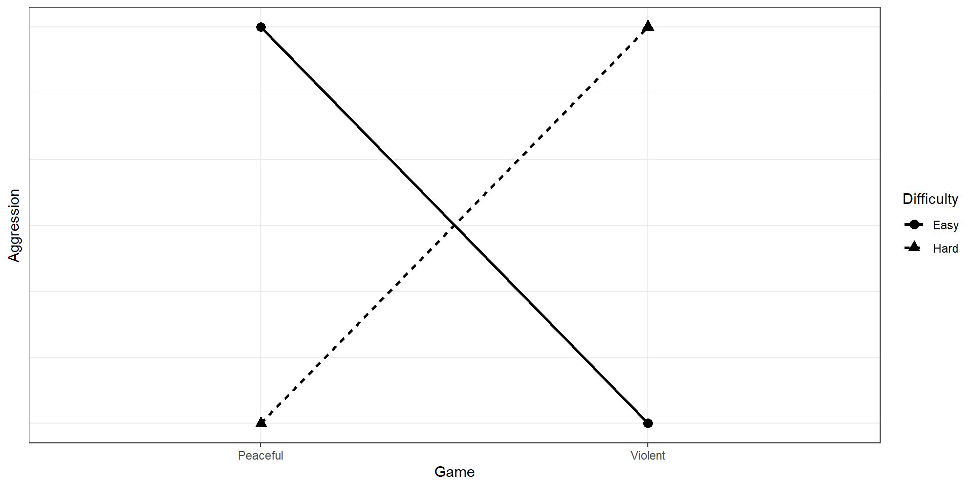
Signif. codes:  0 '***' 0.001 '**' 0.01 '*' 0.05 '.' 0.1 ' ' 1

Aggregating over both conditions means no main effects of either factor. Both conditions have a mean of 1.5:

	Peaceful	Violent
Easy	0	3
Hard	3	0

It gets a bit complicated

• If we don’t go for contrasts, then there’s different types of Sums of Squares for the terms
• Are we interested in only the interaction?
• Do we want to interpret main effects in the presence of an interaction?

What about here?

Yes, there’s main effects: On average, peaceful is lower than violent and on average, easy is lower than difficult. But we know that’s not really the case.

Type I

Sequential sum of squares, where the order of factors matters in unbalanced designs:

• \(SS(A)\)
• \(SS(B | A)\)
• \(SS(AB | B, A)\)

Type II

Presence of Interaction \(SS(AB | A, B)\)? Then no need to test for main effects. If there’s no interaction, then we test main effects.

• \(SS(A |B)\) for factor A
• \(SS(B | A)\) for factor B

Type III

We want everything: Main effects even in the presence of an interaction effect.

• \(SS(A | B, AB)\)
• \(SS(B | A, AB)\)

What do we want?

• With balanced data (same number of observations per cell) none of this matters
• Do we believe main effects are meaningful when there’s an interaction present? If not, Type II are more powerful.
• But our typical hypotheses are about main effects and interaction effects: Type III

Type III

• If we choose to go for Type III, we can’t use dummy coding
• Dummy coding isn’t adequate when there’s interactions present
• Go sum-to-zero instead

Game <- as.factor(d$Game)

contrasts(Game)

  1
0 0
1 1

contrasts(Game) <- contr.sum

contrasts(Game)

  [,1]
0    1
1   -1

Bottom line

• If you have balanced cells, none of this matters
• If you have planned contrasts, none of this matters
• If you have unbalanced cells and care about main effects, you must choose Type III with sum-to-zero contrasts
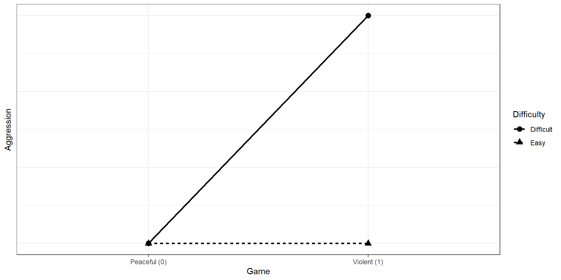
• Either compare models (anova command on two lm models) or go straight to an out-of-the-box ANOVA solutions (e.g., afex package)

Creating unbalanced data

Let’s delete some rows.

rows_to_delete <- sample(nrow(d), 15)
d <- d[-rows_to_delete,]

table(d$Game, d$Difficulty)

   
     0  1
  0 46 46
  1 47 46

Different results

summary(aov(Aggression ~ Game*Difficulty, d))

                 Df Sum Sq Mean Sq F value Pr(>F)    
Game              1    0.9     0.9   1.078  0.301    
Difficulty        1    0.3     0.3   0.306  0.581    
Game:Difficulty   1  412.0   412.0 495.391 <2e-16 ***
Residuals       181  150.5     0.8                   
---
Signif. codes:  0 '***' 0.001 '**' 0.01 '*' 0.05 '.' 0.1 ' ' 1

summary(afex::aov_car(Aggression ~ Game*Difficulty + Error(id), d %>% mutate(id=1:nrow(d)), type = 3))

Anova Table (Type 3 tests)

Response: Aggression
                num Df den Df     MSE        F     ges Pr(>F)    
Game                 1    181 0.83162   0.8505 0.00468 0.3576    
Difficulty           1    181 0.83162   0.4517 0.00249 0.5024    
Game:Difficulty      1    181 0.83162 495.3912 0.73240 <2e-16 ***
---
Signif. codes:  0 '***' 0.001 '**' 0.01 '*' 0.05 '.' 0.1 ' ' 1

The lm solution

• Specify sum-to-zero contrasts
• Run a model with and one without the interaction
• Compare models and get a p-value for just the interaction
• Doesn’t give you the main effects, but fast

The afex solution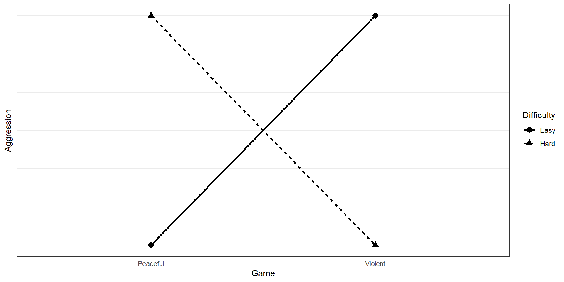

• Needs an ID variable to identify a row
• You can specify the type of tests
• Automatically uses sum-to-zero coding
• Automatically transforms character variables into factors

afex::aov_car(DV ~ IV1*IV2 + Error(ID), data, type = 3)

Power for interactions

• What do I need to power for: The literal interaction effect or will we follow up?
• If we’re not interested in the pattern, then we can just focus on powering for the interaction term
• If we’re interested in the pattern, we must power for simple effects (aka follow-ups)

Same effect size

Full reversal

For full details, see here.

Attentuation

Back to our example

Overall results tells us whether the interaction provides extra information:

# get id variables
d$id <- 1:nrow(d)

# give actual names to factor leves
d$Game <- as.factor(d$Game)
d$Difficulty <- as.factor(d$Difficulty)
levels(d$Game) <- c("Peaceful", "Violent")
levels(d$Difficulty) <- c("easy", "hard")

m <- afex::aov_car(Aggression ~ Game*Difficulty + Error(id), d %>% mutate(id=1:nrow(d)), type = 3)

Back to our example

summary(m)

Anova Table (Type 3 tests)

Response: Aggression
                num Df den Df     MSE        F     ges Pr(>F)    
Game                 1    181 0.83162   0.8505 0.00468 0.3576    
Difficulty           1    181 0.83162   0.4517 0.00249 0.5024    
Game:Difficulty      1    181 0.83162 495.3912 0.73240 <2e-16 ***
---
Signif. codes:  0 '***' 0.001 '**' 0.01 '*' 0.05 '.' 0.1 ' ' 1

Following up

Pairwise comparisons tell us the pattern. Shotgun approach:

pairs(emmeans::emmeans(m, c("Game", "Difficulty")))

 contrast                      estimate    SE  df t.ratio p.value
 Peaceful easy - Violent easy   -3.1084 0.189 181 -16.434  <.0001
 Peaceful easy - Peaceful hard  -3.0748 0.190 181 -16.170  <.0001
 Peaceful easy - Violent hard   -0.2138 0.190 181  -1.124  0.6750
 Violent easy - Peaceful hard    0.0335 0.189 181   0.177  0.9980
 Violent easy - Violent hard     2.8946 0.189 181  15.304  <.0001
 Peaceful hard - Violent hard    2.8610 0.190 181  15.046  <.0001

P value adjustment: tukey method for comparing a family of 4 estimates 

Following up

Pairwise comparisons tell us the pattern. By factor:

pairs(emmeans::emmeans(m, "Game", by = "Difficulty"))

Difficulty = easy:
 contrast           estimate    SE  df t.ratio p.value
 Peaceful - Violent    -3.11 0.189 181 -16.434  <.0001

Difficulty = hard:
 contrast           estimate    SE  df t.ratio p.value
 Peaceful - Violent     2.86 0.190 181  15.046  <.0001

Power for the interaction term

n <- 50
m1 <- 4
m2 <- 4
m3 <- 4
m4 <- 4.5
sd <- 1.5
draws <- 1e3

pvalues <- NULL

for (i in 1:n) {

  group1 <- rnorm(n, m1, sd)
  group2 <- rnorm(n, m2, sd)
  group3 <- rnorm(n, m3, sd)
  group4 <- rnorm(n, m4, sd)

  d <- data.frame(
    id = factor(1:c(4*n)),
    scores = c(group1, group2, group3, group4),
    group1 = factor(rep(c("a", "b"), each = n, times = 2)),
    group2 = factor(rep(c("a", "b"), each = n*2))
  )
  
  contrasts(d$group1) <- contr.sum
  contrasts(d$group2) <- contr.sum
  
  m <- suppressMessages(afex::aov_car(scores ~ group1*group2 + Error(id), data = d, type = 3))
  
  pvalues[i] <- m$anova_table$`Pr(>F)`[3]
}

sum(pvalues < 0.05) / length(pvalues)

[1] 0.2

Takeaways

• Understand what an interaction is from the perspective of the linear model
• Make yourself think in more detail about the form of interactions
• Be able to translate that detail to generating data

Let’s get simulating