Exercise IV

Overview

Once more, this set of exercises won’t introduce new technical skills: You got everything you need for the most common designs. Here, you’ll dive deeper into simulating multiple groups and getting a better feel for how these comparisons work.

0.1 Exercise

ANOVAs are just linear models. There’s nothing wrong with using R’s aov command. In fact, it’s just a wrapper for lm. Type ?aov and convince yourself by reading the (short) description. There’s another reason why directly calling lm can be an advantage: efficiency. So far, we haven’t really cared much about the time our simulations take, but with more complicated designs (or more runs) it can easily take several hours, days, or even weeks.

Let’s see whether lm gives us an advantage. For that, we’ll need the Sys.time() command. It does exactly what it says: tells you the time of your computer system. When we store the time before and after a simulation, we can check how long it took and compare different functions.

Run the following to get familiar with how this works:

t1 <- Sys.time()
# wait a couple of seconds
t2 <- Sys.time()

t2-t1

Now create a data frame with 4 (independent) groups whose means are c(4.2, 4.5, 4.6, 4.6) and their SDs are c(0.7, 0.8, 0.6, 0.5). The sample size is 240 (equal size in the groups). Check for an effect of condition on the outcome in 10,000 simulations. Do that once with aov and once with lm. For each type of model (lm or aov), clock the system time before and after the simulation with Sys.time. Are there differences? (Tip: Remember vectorization for rnorm to create the groups.)

set.seed(42)

means <- c(4.2, 4.5, 4.6, 4.6)
sd <- c(0.7, 0.8, 0.6, 0.5)
n <- 240
runs <- 1e4

# aov run
t1_aov <- Sys.time()

for (i in 1:runs) {
  
  d <- 
    data.frame(
      scores = rnorm(n, means, sd),
      condition = rep(letters[1:4], n/4)
    )
  
  aov(scores ~ condition, d)
}

t2_aov <- Sys.time()

# lm run
t1_lm <- Sys.time()

for (i in 1:runs) {
  
  d <- 
    data.frame(
      scores = rnorm(n, means, sd),
      condition = rep(letters[1:4], n/4)
    )
  
  lm(scores ~ condition, d)
}

t2_lm <- Sys.time()

aov_time <- t2_aov-t1_aov
lm_time <- t2_lm-t1_lm

aov_time-lm_time

Time difference of 1.797944 secs

Expand to get a tip

Did you remember the vectorization? It just means that rnorm will go through vectors in order, such as:

means <- c(4.2, 4.5, 4.6, 4.6)
sd <- c(0.7, 0.8, 0.6, 0.5)
n <- 240
runs <- 1e4

rnorm(n, means, sd

Now all you need to do is put that into a loop (no need to store the results). Just remember to save the time right before and after the loop. Do that once for aov and once for lm; then compare the time differences.

t1_aov <- ?

for (i in 1:?) {
  
  d <- 
    data.frame(
      scores = ?,
      condition = ?
    )
  
  aov(scores ~ condition, d)
}

t2_aov <- ?
  
t2_aov - t1_aov

0.2 Exercise

Time to run a power analysis. You have 3 independent groups. Their means are c(5, 5.2, 5.6); the SD is constant: 1. Your minimum sample size is 120; your maximum sample size is 300. How large does your sample have to be for 95% power? Do 1,000 per run. Go in steps of 6 for the sample size (so increase 2 per group). (Tip: You can use seq and remember this link). This simulation can take a minute (well, several actually).

means <- c(5, 5.2, 5.6)
sd <- 1
sizes <- seq(120, 300, 6)
runs <- 1e3

outcomes <- 
  data.frame(
    sample_size = NULL,
    power = NULL
  )

for (n in sizes) {
  
  pvalues <- NULL
  
  for (i in 1:runs) {
    d <- 
      data.frame(
        scores = rnorm(n, means, sd),
        condition = rep(letters[1:3], n/3)
      )
    
    m <- summary(lm(scores ~ condition, d))
    pvalues[i] <- broom::glance(m)$p.value
  }
  
  outcomes <- 
    rbind(
      outcomes,
      data.frame(
        sample_size = n,
        power = sum(pvalues < 0.05) / length(pvalues)
      )
    )
}

plot(outcomes$sample_size, outcomes$power)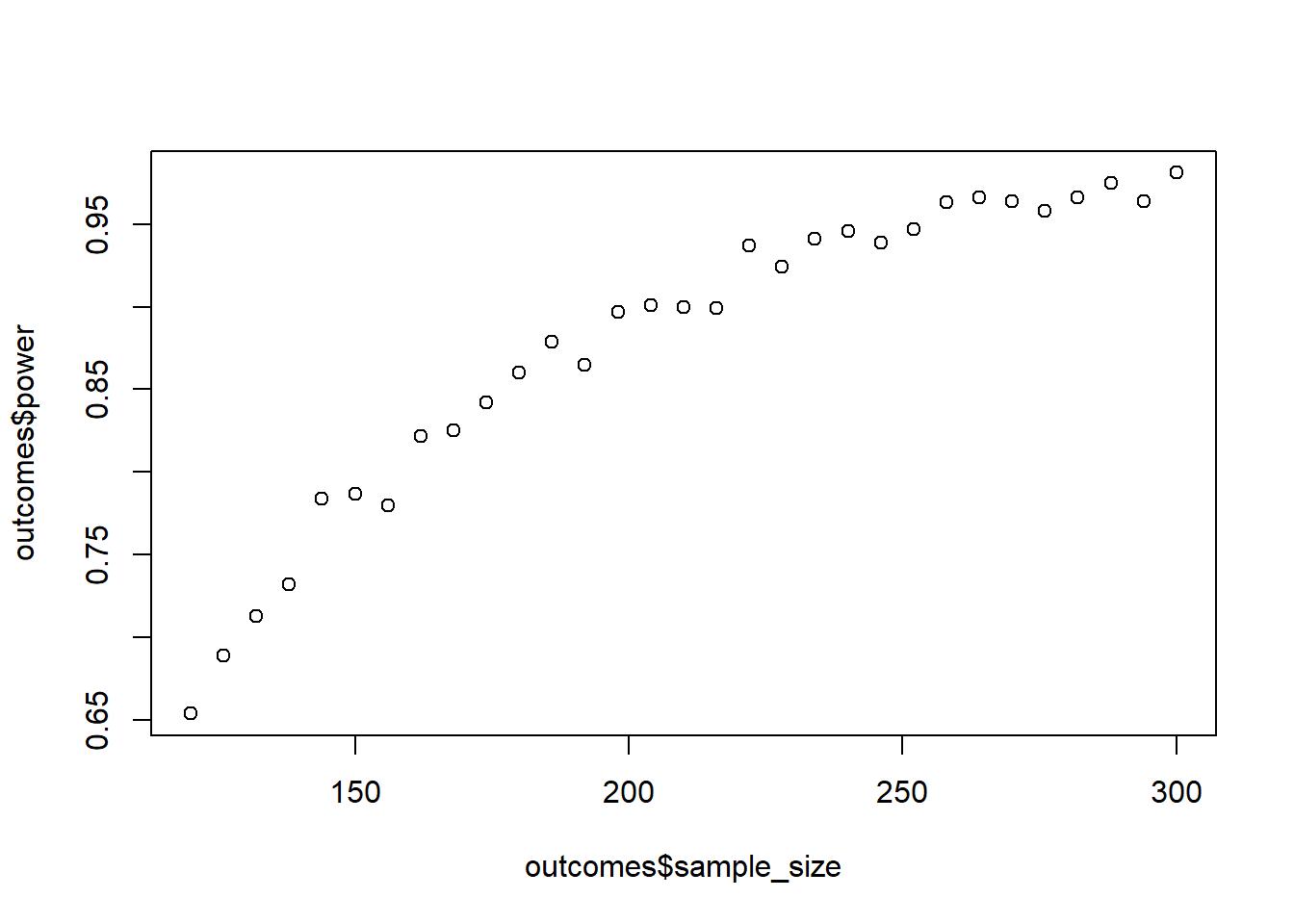

Expand to get a tip

At this point, you’ll know what comes here. We first declare our parameters:

means <- c(5, 5.2, 5.6)
sd <- 1
sizes <- seq(?, ?, ?) # the steps we go up in sample size
runs <- ?

outcomes <- 
  data.frame(
    sample_size = NULL,
    power = NULL
  )

Then we do two loops: On the first level, we iterate over the different sample sizes; on the second level, we iterate over the number of runs. There’s really nothing new here; you can copy-paste code from t-tests and just add another group.

# iterate over the sample sizes
for (? in ?) {
  
  # set up storage for the p-values
  
  # then do the test as many timmes as we decided to do runs
  for (? in 1:?) {
    
    d <- 
      data.frame(
        scores = rnorm(?, ?, ?),
        condition = rep(?, ?)
      )
    
    m <- summary(lm(scores ~ condition, d))
    
    ? <- broom::glance(m)$p.value
  }
  
  # now calculate power and add it to our data frame as always
  outcomes <- 
    rbind(
      outcomes,
      data.frame(
        sample_size = ?,
        power = ?
      )
    )
}

You can plot the power curve with plot(outcomes$sample_size, outcomes$power).

0.3 Exercise

Do the above again, but this time there’s no difference between the first two groups: c(5, 5, 5.6). What’s the effect on power if there’s a null effect for one contrast? Go in steps of 12 to speed it up.

means <- c(5, 5, 5.6)
sd <- 1
sizes <- seq(120, 300, 12)
runs <- 1e3

outcomes <- 
  data.frame(
    sample_size = NULL,
    power = NULL
  )

for (n in sizes) {
  
  pvalues <- NULL
  
  for (i in 1:runs) {
    d <- 
      data.frame(
        scores = rnorm(n, means, sd),
        condition = rep(letters[1:3], n/3)
      )
    
    m <- summary(lm(scores ~ condition, d))
    pvalues[i] <- broom::glance(m)$p.value
  }
  
  outcomes <- 
    rbind(
      outcomes,
      data.frame(
        sample_size = n,
        power = sum(pvalues < 0.05) / length(pvalues)
      )
    )
}

plot(outcomes$sample_size, outcomes$power)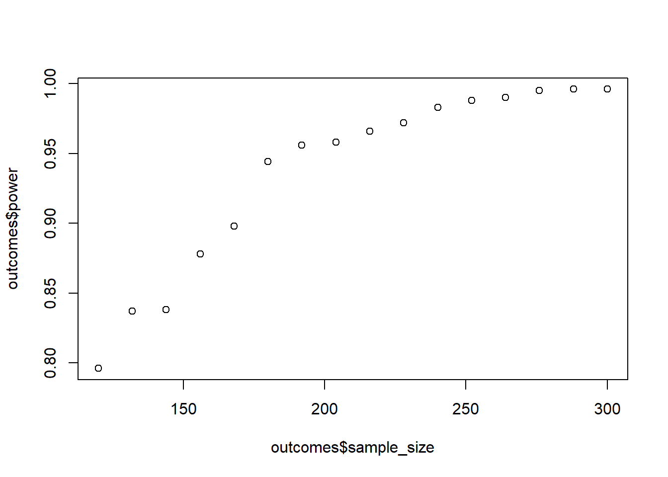

Expand to get a tip

All you need to do is change one number, namely the mean for the second group. The rest of the code is identical to the previous exercise.

0.4 Exercise

Let’s try to work on the standardized scale. You again have 3 groups. Their SDs are c(2, 2.2, 1.8). Choose means such that the Cohen’s $d$s are as follows:

Group 1 vs. Group 2: $d$ = 0.2
Group 1 vs. Group 3: $d$ = 0.6
Group 2 vs. Group 3: ?

Remember the formulate for Cohen’s $d$: $d = \frac{M_1-M_2}{\sqrt{\frac{(sd_1^2 + sd_2^2)}{2}}}$

Have a look at earlier exercises when you dealt with Cohen’s $d$. It might (wink, wink) help to get the pooled SD for each group comparison. Once you have the pooled SD, the absolute means don’t matter as much. You can start with a random mean for the control group, then have the mean for group 2 be the control group mean plus 0.2 pooled SDs (so that we have our Cohen’s $d$). Have a look at earlier exercises on how to calculate the pooled SD. Create a data frame and calculate power for samples ranging from 20 per group to 60 per group. Go in steps of 3 per group. Do 500 runs for each combination. Run effectsize::cohens_d() for each run (and contrast). Store not only the p-values to calculate power, but also the Cohen’s $d$ for each contrast. Plot the power first. Then take the mean of Cohen’s $d$ for each contrast to check whether you actually got the correct numbers.

pooled_sd <- 
  function(sd1, sd2){
    pooled_sd <- sqrt((sd1**2 + sd2**2) / 2)
    
    return(pooled_sd)
  }

sds <- c(2, 2.2, 1.8)

# pooled sd for first two combos (the third is implied when we determine the means)
g1_g2_sd <- pooled_sd(sds[1], sds[2])
g1_g3_sd <- pooled_sd(sds[1], sds[3])

# choose random mean for first group and other groups as proportion of the pooled SD. the last one, logically, has to be 0.4
m1 <- 10
m2 <- m1 + 0.2*g1_g2_sd
m3 <- m1 + 0.6*g1_g3_sd

means <- c(m1, m2, m3)
sizes <- seq(20*3, 60*3, 3*3)
runs <- 500

outcomes <- 
  data.frame(
    sample_size = NULL,
    power = NULL,
    d12 = NULL,
    d13 = NULL,
    d23 = NULL
  )

for (n in sizes) {
  
  pvalues <- NULL
  d12 <- NULL
  d13 <- NULL
  d23 <- NULL
  
  for (i in 1:runs) {
    d <- 
      data.frame(
        scores = rnorm(n, means, sds),
        condition = rep(letters[1:3], n/3)
      )
    
    m <- summary(lm(scores ~ condition, d))
    pvalues[i] <- broom::glance(m)$p.value
    
    # get cohen's for each contrast
    d12[i] <- effectsize::cohens_d(d$scores[d$condition==letters[1]], d$scores[d$condition==letters[2]])$Cohens_d
    d13[i] <- effectsize::cohens_d(d$scores[d$condition==letters[1]], d$scores[d$condition==letters[3]])$Cohens_d
    d23[i] <- effectsize::cohens_d(d$scores[d$condition==letters[2]], d$scores[d$condition==letters[3]])$Cohens_d
  }
  
  outcomes <- 
    rbind(
      outcomes,
      data.frame(
        sample_size = n,
        power = sum(pvalues < 0.05) / length(pvalues),
        d12 = mean(d12),
        d13 = mean(d13),
        d23 = mean(d23)
      )
    )
}

plot(outcomes$sample_size, outcomes$power)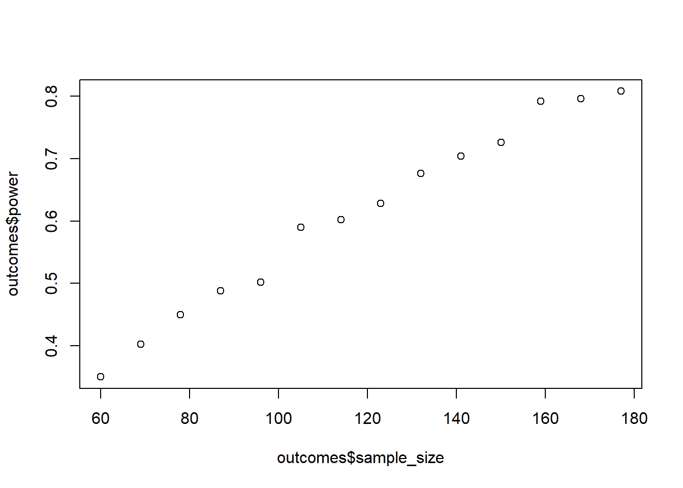

mean(outcomes$d12);mean(outcomes$d13);mean(outcomes$d23)

[1] -0.2022801

[1] -0.6103061

[1] -0.3666429

Expand to get a tip

Alright, first we need a function to get the pooled SD. Afterwards, we get the pooled SD for each contrast.

pooled_sd <- 
  function(sd1, sd2){
    pooled_sd <- ?
    
    return(pooled_sd)
  }

contrast1 <- pooled_sd(2, 2.2)
contrast2 <- pooled_sd(2.2, 3)

That’s really all we need. Now we can pick a random mean and construct the mean of the other groups in relation to that mean plus however many pooled SDs we specified (e.g., 0.2, 0.6).

# choose random mean for first group and other groups as proportion of the pooled SD. the last one, logically, has to be 0.4
mean1 <- ?
mean2 <- m1 + 0.2*?
mean3 <- m1 + 0.6*?

# store the means
means <- c(mean1, mean2, mean3)

# declare the other variables
sizes <- seq(?, ?, ?)
runs <- ?
  
# somewhere to store the results
outcomes <- 
  data.frame(
    sample_size = NULL,
    power = NULL,
    d12 = NULL, # cohen's D for first contrast
    d13 = NULL, # second contrast
    d23 = NULL # third
  )

That’s it. The rest is just lots of typing.

# iterate over sample sizes
for (? in sizes) {
  
  # store p-values and Cohen's ds
  pvalues <- NULL
  d12 <- NULL
  d13 <- NULL
  d23 <- NULL
  
  for (i in 1:runs) {
    d <- 
      data.frame(
        scores = ?,
        condition = ?
      )
    
    m <- summary(lm(? ~ ?, ?))
    pvalues[?] <- broom::glance(?)$?
    
    # get cohen's for each contrast
    d12[i] <- effectsize::cohens_d(?, ?)$Cohens_d
    # etc.
  }
  
  # store it all
  outcomes <- 
    rbind(
      outcomes,
      data.frame(
        sample_size = ?,
        power = ?,
        d12 = mean(d12),
        d13 = ?,
        d23 = ?
      )
    )
}

0.5 Exercise

So far, we’ve worked with dummy coding for our explanatory factor. That presumes that we’re interested in those contrasts where the second and third condition are compared to the first. Sometimes, however, we’re not interested in these comparisons and would rather like to know the difference between our conditions and the grand mean. In that case, we should use sum to zero coding. Take the data set below:

set.seed(42)
n <- 100
d <- 
  data.frame(
    condition = as.factor(rep(letters[1:3], times = n)),
    scores = rnorm(n*3, c(100, 150, 200), c(7, 10, 12))
  )

Let’s have a look at the contrasts:

contrasts(d$condition)

  b c
a 0 0
b 1 0
c 0 1

It’s the familiar dummy coding. This means, going row by row, that, to get the mean for a, both b and c estimates will be zero. When everything is zero, that’s our intercept. In other words, the intercept will be the mean of condition a. To get b, we take the intercept plus 1 times the b estimate (mean of condition b in comparison to a), and to get c, we take the intercept plus 1 time the estimate for c (aka the mean of c in comparison to a).

Let’s have a look at contrast coding instead:

contrasts(d$condition) <- contr.sum
contrasts(d$condition)

  [,1] [,2]
a    1    0
b    0    1
c   -1   -1

Now the intercept is our grand mean (the overall mean of the outcome), the first contrast compares the score in condition a against the grand mean and the second contrast compares the mean of condition b against the grand mean. To get c, we need to take the intercept take the estimate of a times -1 plus the estimate of c times -1 (so grand mean minus a and minus b).

summary(lm(scores~condition, d))


Call:
lm(formula = scores ~ condition, data = d)

Residuals:
    Min      1Q  Median      3Q     Max 
-32.364  -6.417  -0.009   6.081  26.953 

Coefficients:
            Estimate Std. Error t value Pr(>|t|)    
(Intercept) 149.8348     0.5700 262.872   <2e-16 ***
condition1  -50.0140     0.8061 -62.045   <2e-16 ***
condition2   -0.6376     0.8061  -0.791     0.43    
---
Signif. codes:  0 '***' 0.001 '**' 0.01 '*' 0.05 '.' 0.1 ' ' 1

Residual standard error: 9.873 on 297 degrees of freedom
Multiple R-squared:  0.946, Adjusted R-squared:  0.9456 
F-statistic:  2600 on 2 and 297 DF,  p-value: < 2.2e-16

If we want a different comparison, we can reorder the factor levels:

d$condition <- factor(d$condition, levels = c("b", "c", "a")) 
contrasts(d$condition) <- contr.sum
contrasts(d$condition)

  [,1] [,2]
b    1    0
c    0    1
a   -1   -1

Now the first contrasts compares condition b against the grand mean, and the second contrast compares condition c against the grand mean.

For later sessions on interactions, we’ll rely on this kind of sum-to-zero coding (also called effect coding), so let’s get familiar with it here. Create four groups: a placebo group, a low dose group, a medium dose group, and a high dose group.

You want to know whether the low dose, the medium dose, and the high dose are significantly different from the grand mean. Simulate a data set, set the contrasts, and run a linear model. Choose mean values as you like, but make sure you can find them again in the model output. Speaking of the model output: How would you get the mean of the placebo group now? How would you get the mean of any group? (Tip: Look at the contrasts (aka the estimates from the model), take the grand mean, and apply the contrasts to each estimate.)

n <- 50
d <- 
  data.frame(
    condition = factor(rep(c("placebo", "low dose", "medium dose", "high dose"), times = n)),
    scores = rnorm(n*4, c(10, 20, 30, 40), 2)
  )

d$condition <- factor(d$condition, levels = c("low dose", "medium dose", "high dose", "placebo"))
contrasts(d$condition) <- contr.sum
contrasts(d$condition)

            [,1] [,2] [,3]
low dose       1    0    0
medium dose    0    1    0
high dose      0    0    1
placebo       -1   -1   -1

summary(lm(scores ~ condition, d))


Call:
lm(formula = scores ~ condition, data = d)

Residuals:
    Min      1Q  Median      3Q     Max 
-4.3991 -1.2198 -0.1447  1.3646  5.5612 

Coefficients:
            Estimate Std. Error t value Pr(>|t|)    
(Intercept)  24.9151     0.1334  186.74   <2e-16 ***
condition1   -5.4787     0.2311  -23.71   <2e-16 ***
condition2    5.4555     0.2311   23.61   <2e-16 ***
condition3   14.9170     0.2311   64.55   <2e-16 ***
---
Signif. codes:  0 '***' 0.001 '**' 0.01 '*' 0.05 '.' 0.1 ' ' 1

Residual standard error: 1.887 on 196 degrees of freedom
Multiple R-squared:  0.9731,    Adjusted R-squared:  0.9726 
F-statistic:  2360 on 3 and 196 DF,  p-value: < 2.2e-16

# get placebo mean
coefs <- coef(lm(scores ~ condition, d))
coefs[1] + sum(coefs[-1] * contrasts(d$condition)["placebo", ])

(Intercept) 
   10.02139

Expand to get a tip

There’s nothing complicated here. We’re only doing one run. So first you create a data frame and choose a sample size and some means (feel free to choose any):

n <- 50
d <- 
  data.frame(
    condition = factor(rep(c("placebo", "low dose", "medium dose", "high dose"), times = n)),
    scores = rnorm(n*4, c(?, ?, ?, ?), 2)
  )

Then let’s code the contrasts:

d$condition <- factor(d$condition, levels = c("low dose", "medium dose", "high dose", "placebo")) # rearrange the levels
contrasts(d$condition) <- contr.sum # apply sum-to-zero contrasts
contrasts(d$condition) # have a look

Then all that’s left is to run an lm model. To get the placebo mean you need to take the grand mean and then subtract each estimate from it (remember that minus a negative estimate means adding).

0.6 Exercise

You plan an experiment where you want to test the effect of framing on agreeing with a message. In your experiment people read a text with either neutral, positive, or negative framing. Each person reads each text (so we have a within-subjects design) and rates their level of agreeing on a 7-point Likert-scale.

You determine that the smallest contrast you care about is 0.25 points between the neutral and the negative condition and between the neutral and the positive condition. You’ve found in previous testing that only such a difference on agreeing actually has an effect on behavior. That’s your SESOI.

You decide that the midpoint of the scale is a decent starting point for the neutral condition. The negative condition should be 0.25 points lower and the positive condition 0.25 points higher. You generally expect that the variation should be somewhere around 1 Likert-point; this way, most scores are within -2 and +2 from the mean. However, you know that negative framing usually increases variation, so you’ll set the SD for that score 30% higher than that of the other two conditions.

The experiment takes place within 20 minutes, so you expect a decent amount of consistency in answers per participant: a person who generally agrees more should also agree more to all conditions. In other words, you set the correlation between scores to 0.6.

Last, you determined that you’re early in the research process, so you definitely don’t want to miss any effects (aka commit a Type II error). You also consider that a false positive won’t have any negative consequences. Therefore, you set your $\alpha$ to 0.10.

You can afford to collect 100 participants in total (that’s where you’ll stop with the simulation). Simulate power (500 runs each); go in steps of 5 (start with 20). How many participants do you need for 95% power? Will 100 even get you there? Use contrast coding.

Several tips:

For the variance-covariance matrix, you’ll need to get different covariances based on the groups
Remember the data format the data have to be in. You’ll need to transform them from wide to long format. Have a look at the slides or good old Google
You might have to Google how to get the p-value out of aov (one method that worked for me was unlist(model)["Error: Within.Pr(>F)1"])

library(MASS)
library(tidyr)

means <- c(neutral = 4, negative = 3.75, positive = 4.25)
sd_neutral_po <- 1
sd_negative <- 1.3
correlation <- 0.6
sizes <- seq(10, 100, 5)
runs <- 500
alpha <- 0.10

# covariance for negative with the two others is identical because the sd for the other two is identical
cov_negative <- correlation * sd_neutral_po * sd_negative
cov_other <- correlation * sd_neutral_po * sd_neutral_po

our_matrix <- matrix(
  c(
    sd_neutral_po**2, cov_negative, cov_other,
    cov_negative, sd_negative**2, cov_negative,
    cov_other, cov_negative, sd_neutral_po**2
  ),
  ncol = 3
)

outcomes <- 
  data.frame(
    sample_size = NULL,
    power = NULL
  )

for (n in sizes) {
  
  pvalues <- NULL
  
  for (i in 1:runs) {
    d <- mvrnorm(
      n,
      means,
      our_matrix
    )
    
    d <- as.data.frame(d)
    d$id <- factor(1:n)
    
    d <- pivot_longer(
      d,
      cols = -id,
      values_to = "scores",
      names_to = "condition"
    )
    
    d$condition <- as.factor(d$condition)
    
    contrasts(d$condition) <- contr.sum
    
    m <- summary(aov(scores ~ condition + Error(id), d))
    
    pvalues[i] <- unlist(m)["Error: Within.Pr(>F)1"]
  }
  
  outcomes <- 
    rbind(
      outcomes,
      data.frame(
        sample_size = n,
        power = sum(pvalues < alpha) / length(pvalues)
      )
    )
}

plot(outcomes$sample_size, outcomes$power)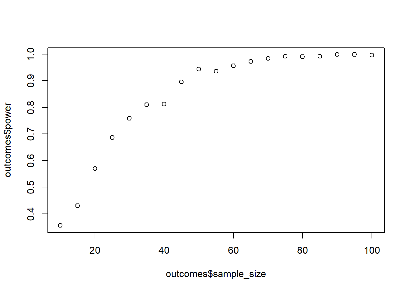

Expand to get a tip

The complication here really comes from the variance-covariance matrix. This time, you can’t use the same covariance between groups because the variances differ per group. But before we get there, let’s first declare our variables. That should help:

library(MASS)
library(tidyr)

means <- c(neutral = ?, negative = ?, positive = ?)
sd_neutral_po <- ?  # the SD for the neutral and positive conditions
sd_negative <- ? # the SD for the negative conditions
correlation <- ? # the correlation between conditions
sizes <- seq(?, ?, ?) # in what steps will we go up in sample size?
runs <- ?
alpha <- ? # our Type I error rate

Once we have all of that, we need to construct the variance-covariance matrix. Because negative condition is different from the positive and neutral conditions, we’ll need to create a covariance especially covariances between negative and the other two, as well as a covariance between neutral and positive

# covariance for negative with the two others is identical because the sd for the other two is identical
cov_negative <- correlation * ? * ? # correlation times SD for neutral/positive times SD for negative
cov_other <- correlation * ? * ? # correlation times SD for neutral/positive times SD for neutral/positive again

# then we create the matrix
our_matrix <- matrix(
  c(
    sd_neutral_po**2, cov_negative, cov_other,
    cov_negative, sd_negative**2, cov_negative,
    cov_other, cov_negative, sd_neutral_po**2
  ),
  ncol = 3
)

# somewhere to store our outcomes
outcomes <- 
  data.frame(
    sample_size = NULL,
    power = NULL
  )

Now that we have out variance-covariance matrix, we can go to the actual simulations. We iterate over sample sizes, create normal scores, transform those into the long format (see the slides for code), and run the Repeated-Measures ANOVA.

# iterate over sample sizes
for (? in ?) {
  
  # somewhere to store the p-values
  pvalues <- NULL
  
  for (i in 1:runs) {
    d <- mvrnorm(
      ?,
      ?,
      ?
    )
    
    # turn d into the long format
    
    # then assign sum-to-zero contrasts
    contrasts(d$condition) <- contr.sum
    
    # get the condition effect
    m <- summary(aov(scores ~ condition + Error(id), d))
    
    # and store it
    pvalues[i] <- unlist(m)["Error: Within.Pr(>F)1"]
  }
  
  outcomes <- 
    rbind(
      outcomes,
      data.frame(
        sample_size = ?,
        power = ?
      )
    )
}

You can plot the results with plot(outcomes$sample_size, outcomes$power).

0.7 Exercise

The previous study worked. Nice. Now you want to know whether positive framing scales: Can you reduce positivity and agreeing reduces proportionally? You run a follow-up experiment where you now have a neutral condition, a low positivity condition (half the positivity of your previous positive condition), and a high positivity condition (the positivity of your original positive condition). Your effect size remains: 0.25 for the comparison between neutral and high positivity (the original positive condition). You expect, therefore, that half the positivity should lead to half the effect size: 0.125. That’s your new SESOI.

The previous study also showed that you weren’t too far off with an SD of 1, but this time you’ll use 0.8 for all scores.

However, you expect that, because the two positivity conditions are so similar, they’ll correlate higher than the correlation between neutral and positivity. So you expect a correlation between neutral and either positivity condition to be 0.3, but 0.6 between the two positivity conditions.

Because your department was so happy with how well you designed the previous study, they gave you more money. Now you can collect a maximum of 500 participants. Last time, the power simulation took quite some time, so this time you want to stop whenever you reach 95% power (while). Also, because this time you want to be more stringent, you set $\alpha$ to 0.01.

Do 500 runs, start with 60 people and go in in steps of 10. Use treatment contrasts. This can take a while.

library(MASS)
library(tidyr)

set.seed(42)

sesoi <- 0.125
means <- c(neutral = 4, low = 4+sesoi, high = 4+2*sesoi)
sd <- 0.8
cor_positive <- 0.6
cor_neutral <- 0.3
runs <- 500
alpha <- 0.01
max_n <- 500
steps <- 10

# covariance for neutral with the two others is identical because the SD and correlation for the other two is identical
cov_positive <- cor_positive * sd * sd
cov_neutral <- cor_neutral * sd * sd

our_matrix <- matrix(
  c(
    sd**2, cov_neutral, cov_neutral,
    cov_neutral, sd**2, cov_positive,
    cov_neutral, cov_positive, sd**2
  ),
  ncol = 3
)

outcomes <- 
  data.frame(
    sample_size = NULL,
    power = NULL
  )

power <- 0
n <- 60

while (power < 0.95 & n <= max_n) {
  
  pvalues <- NULL
  
  for (i in 1:runs) {
    
    d <- mvrnorm(
      n,
      means,
      our_matrix
    )
    
    d <- as.data.frame(d)
    
    d$id <- factor(1:n)
    
    d <- pivot_longer(
      d,
      cols = -id,
      values_to = "scores",
      names_to = "condition"
    )
    
    d$condition <- as.factor(d$condition)
    
    m <- summary(aov(scores ~ condition + Error(id), d))
    
    pvalues[i] <- unlist(m)["Error: Within.Pr(>F)1"]
  }
  
  power <- sum(pvalues < alpha) / length(pvalues)
  
  outcomes <- 
  rbind(
    outcomes,
    data.frame(
      sample_size = n,
      power = power
    )
  )
  
  n <- n + steps
}
  
plot(outcomes$sample_size, outcomes$power)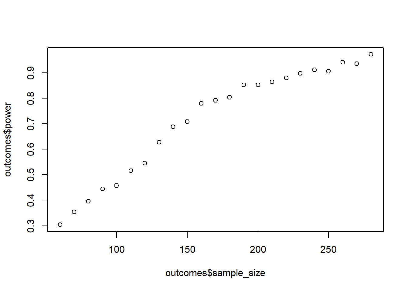

Expand to get a tip

Okay, nothing new here, just a lot. Let’s do the easy stuff first: Declare variables.

library(MASS)
library(tidyr)

sesoi <- ?
means <- c(neutral = 4, low = 4+sesoi, high = 4+2*sesoi)
sd <- ?
cor_positive <- ? # the correlation between positive conditions
cor_neutral <- ? # the correlation between neutral and either positive condition
runs <- ?
alpha <- ?
max_n <- ? # maximum number of participants
steps <- ? # in what steps are you going up?

Okay, this time when constructing the variance-covariance matrix, the SD will be the same, but the correlation will differ. Therefore, we need to create a covariance for neutral with either positivity condition

# covariance for negative with the two others is identical because the sd for the other two is identical
cov_positive <- ? * sd * sd # covariance of positive with the other positive
cov_neutral <- ? * sd * sd # covariance of neutral with either positive

our_matrix <- matrix(
  c(
    sd**2, cov_neutral, cov_neutral,
    cov_neutral, sd**2, cov_positive,
    cov_neutral, cov_positive, sd**2
  ),
  ncol = 3
)

# somewhere to store our outcomes
outcomes <- 
  data.frame(
    sample_size = NULL,
    power = NULL
  )

Now that we have out variance-covariance matrix, we can go to the actual simulations once more. We continue running 500 simulations for a given sample size step unless we reach 95% power or our maximum number of participants.

power <- ? # starting power
n <- ? # starting sample size

while (power < ? & n <= ?) {
  
  # store p-values somewhere
  pvalues <- NULL
  
  # do the 500 simulations for this sample size
  for (i in 1:runs) {
    
    d <- mvrnorm(
      ?,
      ?,
      ?
    )
    
    # transform to long form
    d <- as.data.frame(d)
    
    d$id <- factor(1:n)
    
    d <- pivot_longer(
      d,
      cols = -id,
      values_to = "scores",
      names_to = "condition"
    )
    
    d$condition <- as.factor(d$condition)
    
    # run model
    m <- summary(aov(? ~ ? + Error(?), ?))
    
    # get p-values
  }
  
  power <- ?
  
  # add to results
  outcomes <- 
  rbind(
    outcomes,
    data.frame(
      sample_size = n,
      power = power
    )
  )
  
  # increase sample size
  n <- ?
}

0.8 Exercise

Usually when you run an ANOVA, you specify your contrasts before-hand so you know which groups you want to compare beyond just the overall effect of your condition. Let’s take the data set below. The overall effect of condition is significant:

library(MASS)
library(tidyr)

set.seed(42)

means <- c(neutral = 10, low = 12, high = 14)
sd <- 8
correlation <- 0.6
n <- 80

covariance <- correlation * sd * sd

sigma <- matrix(
  c(
    sd**2, covariance, covariance,
    covariance, sd**2, covariance,
    covariance, covariance, sd**2
  ),
  ncol = 3
)

d <- data.frame(
  mvrnorm(
    n,
    means,
    sigma
  )
)

d$id <- factor(1:n)
    
d <- pivot_longer(
  d,
  cols = -id,
  values_to = "scores",
  names_to = "condition"
)

d$condition <- as.factor(d$condition)

m <- aov(scores ~ condition + Error(id), d)

summary(m)


Error: id
          Df Sum Sq Mean Sq F value Pr(>F)
Residuals 79  12853   162.7               

Error: Within
           Df Sum Sq Mean Sq F value   Pr(>F)    
condition   2    606  303.22   14.23 2.07e-06 ***
Residuals 158   3366   21.31                     
---
Signif. codes:  0 '***' 0.001 '**' 0.01 '*' 0.05 '.' 0.1 ' ' 1

Let’s inspect the post-hoc comparisons between the groups with the emmeans package. Here, not every comparison is significant.

posthocs <- emmeans::emmeans(m, ~ condition)
posthocs

 condition emmean    SE  df lower.CL upper.CL
 high       13.55 0.925 122     11.7     15.4
 low        12.30 0.925 122     10.5     14.1
 neutral     9.73 0.925 122      7.9     11.6

Warning: EMMs are biased unless design is perfectly balanced 
Confidence level used: 0.95

pairs(posthocs)

 contrast       estimate   SE  df t.ratio p.value
 high - low         1.25 0.73 158   1.713  0.2035
 high - neutral     3.82 0.73 158   5.232  <.0001
 low - neutral      2.57 0.73 158   3.519  0.0016

P value adjustment: tukey method for comparing a family of 3 estimates

Run a power simulation that finds the sample size for which we have 90% power for the smallest post-hoc contrast (aka the largest of the three p-values.) Go about it as you think is best, but save both the main effect p-value and the largest p-value of the posthoc contrasts to be able to compare power. In effect, you’re powering for a t-test, which only emphasizes that you should work on the raw scale and specify each comparison. (Tip: summary turns the pairs(postdocs) into a data frame.)

means <- c(neutral = 10, low = 12, high = 14)
sd <- 8
correlation <- 0.6
n <- 20
draws <- 1e3

covariance <- correlation * sd * sd

sigma <- matrix(
  c(
    sd**2, covariance, covariance,
    covariance, sd**2, covariance,
    covariance, covariance, sd**2
  ),
  ncol = 3
)

outcomes <- data.frame(
  sample_size = NULL,
  power = NULL,
  power_posthoc = NULL
)

power_posthoc <- 0

while (power_posthoc < .90) {
  
  pvalues_posthoc <- NULL
  pvalues <- NULL
  
  for (i in 1:runs) {
    
    d <- data.frame(
      mvrnorm(
        n,
        means,
        sigma
      )
    )
    
    d$id <- factor(1:n)
        
    d <- pivot_longer(
      d,
      cols = -id,
      values_to = "scores",
      names_to = "condition"
    )
    
    d$condition <- as.factor(d$condition)
    
    m <- aov(scores ~ condition + Error(id), d)
    
    pvalues[i] <- unlist(summary(m))["Error: Within.Pr(>F)1"]
    
    posthocs <- suppressMessages(emmeans::emmeans(m, ~ condition))
    outputs <- summary(pairs(posthocs))
    
    pvalues_posthoc[i] <- max(outputs$p.value)
  }
  
  power <- sum(pvalues < 0.05) / length(pvalues)
  power_posthoc <- sum(pvalues_posthoc < 0.05) / length(pvalues_posthoc)
  
  outcomes <- 
    rbind(
      outcomes,
      data.frame(
        sample_size = n,
        power = power,
        power_posthoc = power_posthoc
      )
    )
  
  n <- n + 10
}

library(ggplot2)

outcomes %>% 
  pivot_longer(
    cols = starts_with("power"),
    names_to = "Power Type"
  ) %>% 
  ggplot(
    aes(x = sample_size, y = value, color = `Power Type`)
  ) +
  geom_line() + theme_bw()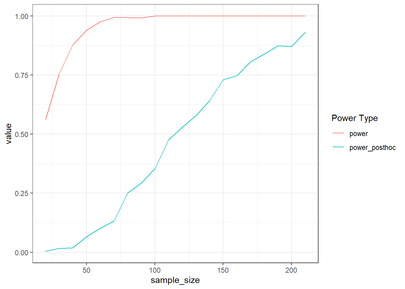

Expand to get a tip

Okay, nothing new here, just a lot. Let’s do the easy stuff first: Declare variables.

library(MASS)
library(tidyr)

sesoi <- ?
means <- c(neutral = 4, low = 4+sesoi, high = 4+2*sesoi)
sd <- ?
cor_positive <- ? # the correlation between positive conditions
cor_neutral <- ? # the correlation between neutral and either positive condition
runs <- ?
alpha <- ?
max_n <- ? # maximum number of participants
steps <- ? # in what steps are you going up?

This time when constructing the variance-covariance matrix, the SD will be the same, but the correlation will differ. Therefore, we need to create a covariance for neutral with either positivity condition

# covariance for negative with the two others is identical because the sd for the other two is identical
cov_positive <- ? * sd * sd # covariance of positive with the other positive
cov_neutral <- ? * sd * sd # covariance of neutral with either positive

our_matrix <- matrix(
  c(
    sd**2, cov_neutral, cov_neutral,
    cov_neutral, sd**2, cov_positive,
    cov_neutral, cov_positive, sd**2
  ),
  ncol = 3
)

# somewhere to store our outcomes
outcomes <- 
  data.frame(
    sample_size = NULL,
    power = NULL
  )

power <- ? # starting power
n <- ? # starting sample size

while (power < ? & n <= ?) {
  
  # store p-values somewhere
  pvalues <- NULL
  
  # do the 500 simulations for this sample size
  for (i in 1:runs) {
    
    d <- mvrnorm(
      ?,
      ?,
      ?
    )
    
    # transform to long form
    d <- as.data.frame(d)
    
    d$id <- factor(1:n)
    
    d <- pivot_longer(
      d,
      cols = -id,
      values_to = "scores",
      names_to = "condition"
    )
    
    d$condition <- as.factor(d$condition)
    
    # run model
    m <- summary(aov(? ~ ? + Error(?), ?))
    
    # get p-values
    pvalues[i] <- ?
    
      # get the posthoc comparisons
    posthocs <- suppressMessages(emmeans::emmeans(m, ~ condition))
    
    # turn into a data frame we can access
    outputs <- summary(pairs(posthocs))
    
    # then get the largest p-value of the contrasts
    pvalues_posthoc[i] <- ?
  }
  
  power <- ?
  
  # add to results
  outcomes <- 
  rbind(
    outcomes,
    data.frame(
      sample_size = n,
      power = power
    )
  )
  
  # increase sample size for the next round of the while statement
  n <- ?
}

0.9 Exercise

Rather than doing posthoc comparisons between each group, we can rely on planned contrasts. If that’s completely new to you, have a read here. The blog post does a really nice job explaining planned contrasts.

In effect, rather than relying on sum to zero or treatment coding, we create our own comparisons. Let’s say we want to compare neutral to both low positivity and high positivity (as a general test that framing works). Then, our second contrast compares the two framing conditions. For simplicity, let’s go three independent groups with means of c(4, 4.3, 4.4) and a common SD of 1.1. Custom contrasts will allow us to directly make the two comparisons we’re interested in like such:

d <- data.frame(
  scores = rnorm(150, c(4, 4.3, 4.4), 1.1),
  condition = factor(rep(c("neutral", "low", "high"), 50))
)

contrasts(d$condition)

        low neutral
high      0       0
low       1       0
neutral   0       1

highlow_vs_neutral <- c(1, 1, -2)
high_vs_low <- c(1, -1, 0)

contrasts(d$condition) <- cbind(highlow_vs_neutral, high_vs_low)
contrasts(d$condition)

        highlow_vs_neutral high_vs_low
high                     1           1
low                      1          -1
neutral                 -2           0

summary.lm(aov(scores ~ condition, d))


Call:
aov(formula = scores ~ condition, data = d)

Residuals:
     Min       1Q   Median       3Q      Max 
-2.97137 -0.80870 -0.03995  0.77749  2.70410 

Coefficients:
                            Estimate Std. Error t value Pr(>|t|)    
(Intercept)                  4.26182    0.08776  48.562   <2e-16 ***
conditionhighlow_vs_neutral  0.13517    0.06206   2.178    0.031 *  
conditionhigh_vs_low         0.09555    0.10748   0.889    0.375    
---
Signif. codes:  0 '***' 0.001 '**' 0.01 '*' 0.05 '.' 0.1 ' ' 1

Residual standard error: 1.075 on 147 degrees of freedom
Multiple R-squared:  0.03629,   Adjusted R-squared:  0.02318 
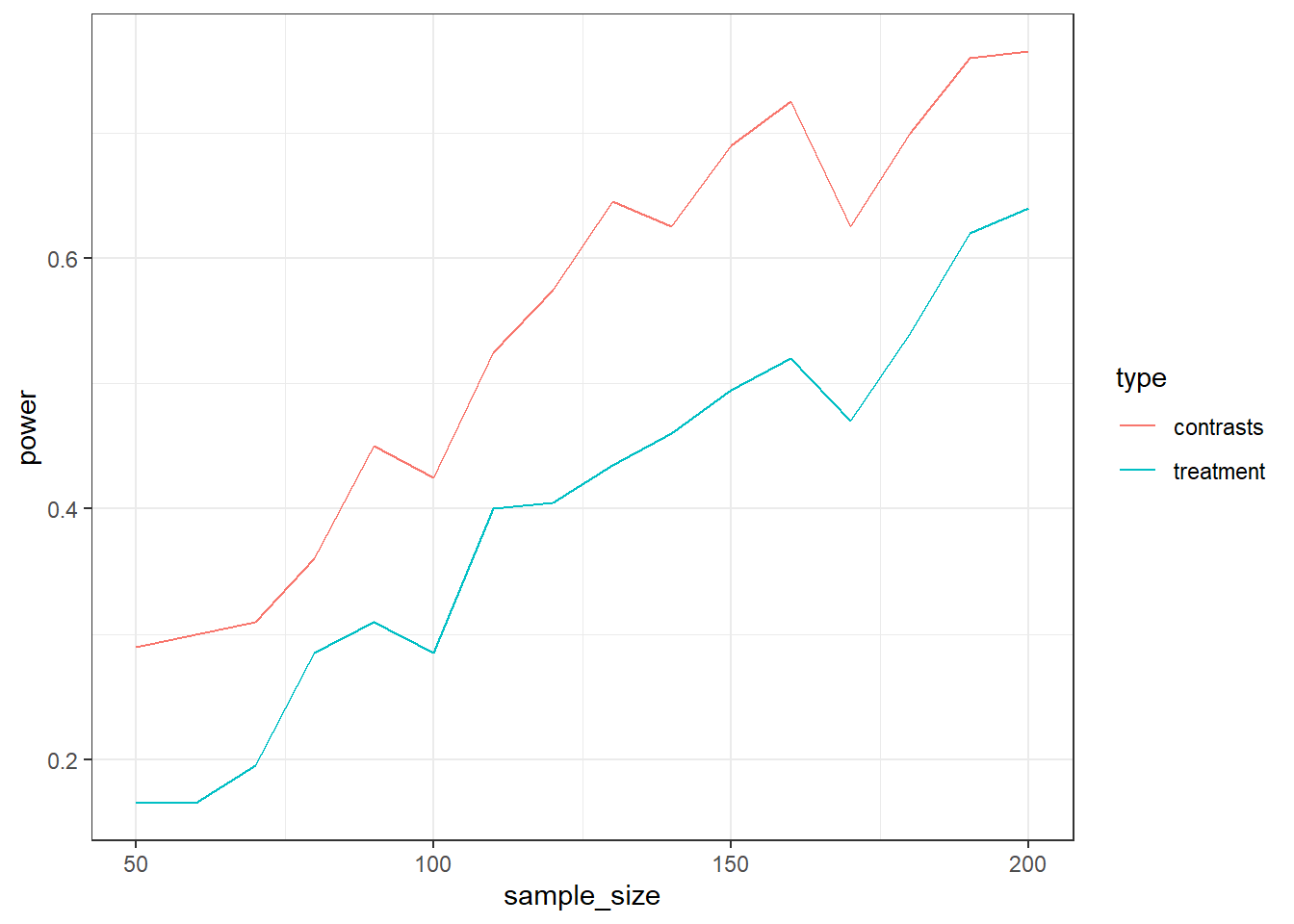
F-statistic: 2.768 on 2 and 147 DF,  p-value: 0.06609

Run a power simulation where you first run standard treatment contrasts. Then, run posthoc tests (emmeans::emmeans) on that test. For simplicity, focus on the comparison of high vs. low. Select the p-value for that posthoc contrast. In the same run, change the contrasts to custom from above, run the model again, and extract the p-value for the high vs. low comparison. Do that for samples ranging from 50 to 200 in steps of 10. Do 200 runs to save a bit of time, then plot the two types of power against each other. Which approach is more “powerful”? No tips here–see this as a little challenge.

set.seed(42)

means <- c(4., 4.3, 4.6)
sd <- 1.1
runs <- 200
sizes <- seq(50, 200, 10)

outcomes <- 
  data.frame(
    sample_size = NULL,
    type = NULL,
    power = NULL
  )

for (n in sizes) {
  pvalues_treatment <- NULL
  pvalues_contrasts <- NULL
  
  for (i in 1:runs) {
    d <- data.frame(
      scores = rnorm(n*3, means, 1.1),
      condition = factor(rep(c("neutral", "low", "high"), n))
    )
    posthocs <- suppressMessages(emmeans::emmeans(lm(scores~condition, d), ~ condition))
    outputs <- summary(pairs(posthocs))
    
    pvalues_treatment[i] <- outputs[1,6]
    
    highlow_vs_neutral <- c(1, 1, -2)
    high_vs_low <- c(1, -1, 0)
    contrasts(d$condition) <- cbind(highlow_vs_neutral, high_vs_low)
    
    pvalues_contrasts[i] <- coefficients(summary(lm(scores~condition, d)))[3,4]
  }
  
  outcomes <- 
    rbind(
      outcomes,
      data.frame(
        sample_size = c(n, n),
        type = c("treatment", "contrasts"),
        power = c(
          sum(pvalues_treatment < 0.05) / length(pvalues_treatment),
          sum(pvalues_contrasts < 0.05) / length(pvalues_contrasts)
        )
      )
    )
}

ggplot(outcomes, aes(x = sample_size, y = power, color = type)) + geom_line() + theme_bw()