library(ggplot2)

ggplot(outcomes, aes(x = sample_size, y = power, color = type)) + geom_line() + theme_bw()Exercise VI
Overview
You made it: last set of exercises. Nothing new here; just an extension of the skills you already have at this point. You’ll simulate power for continuous predictors and interactions.
0.1 Exercise
You’re interested in the effects of three predictors on an outcome. When all predictors are 0, the outcome (y) should be around 16. The first predictor, x1, causes a 1-point increase in y; the second predictor, x2 causes a 0.3-point increase in y; the third predictor, x3, causes a 1.4 increase in y. All predictors range from 0 to 7; for our purposes, we can assume that they’re uniformly distributed. The error term has a mean of 0 and an SD of 10.
Simulate power with 500 runs. You could either power for the entire model (so for the p-value of the F-test for the full lm model) or for each individual predictor. Find out which has the most power: Store power for the full model and each individual predictor from the model. Start with 50 participants and go up in steps of 10 until you reach 200. Plot the power curves for the different power types. You can use the code below:
set.seed(42)

b0 <- 16
b1 <- 1
b2 <- 0.3
b3 <- 1.4
sizes <- seq(50, 200, 10)
runs <- 500

outcomes <-
  data.frame(
    sample_size = NULL,
    type = NULL,
    power = NULL
  )

for (n in sizes) {

  pvalues_all <- NULL
  pvalues_x1 <- NULL
  pvalues_x2 <- NULL
  pvalues_x3 <- NULL

  for (i in 1:runs) {

    error <- rnorm(n, 0, 10)

    x1 <- runif(n, 0, 7)
    x2 <- runif(n, 0, 7)
    x3 <- runif(n, 0, 7)

    d <-
      data.frame(
        x1 = x1,
        x2 = x2,
        x3 = x3,
        y = b0 + b1*x1 + b2*x2 + b3*x3 + error
      )

    m <- summary(lm(y ~ x1 + x2 + x3, d))

    pvalues_all[i] <- broom::glance(m)$p.value
    pvalues_x1[i] <- broom::tidy(m)$p.value[2]
    pvalues_x2[i] <- broom::tidy(m)$p.value[3]
    pvalues_x3[i] <- broom::tidy(m)$p.value[4]
  }

  outcomes <-
    rbind(
      outcomes,
      data.frame(
        sample_size = rep(n, 4),
        type = factor(c("all", "x1", "x2", "x3")),
        power = c(
          sum(pvalues_all < 0.05) / length(pvalues_all),
          sum(pvalues_x1 < 0.05) / length(pvalues_x1),
          sum(pvalues_x2 < 0.05) / length(pvalues_x2),
          sum(pvalues_x3 < 0.05) / length(pvalues_x3)
        )
      )
    )
}

library(ggplot2)
ggplot(outcomes, aes(x = sample_size, y = power, color = type)) + geom_line() + theme_bw()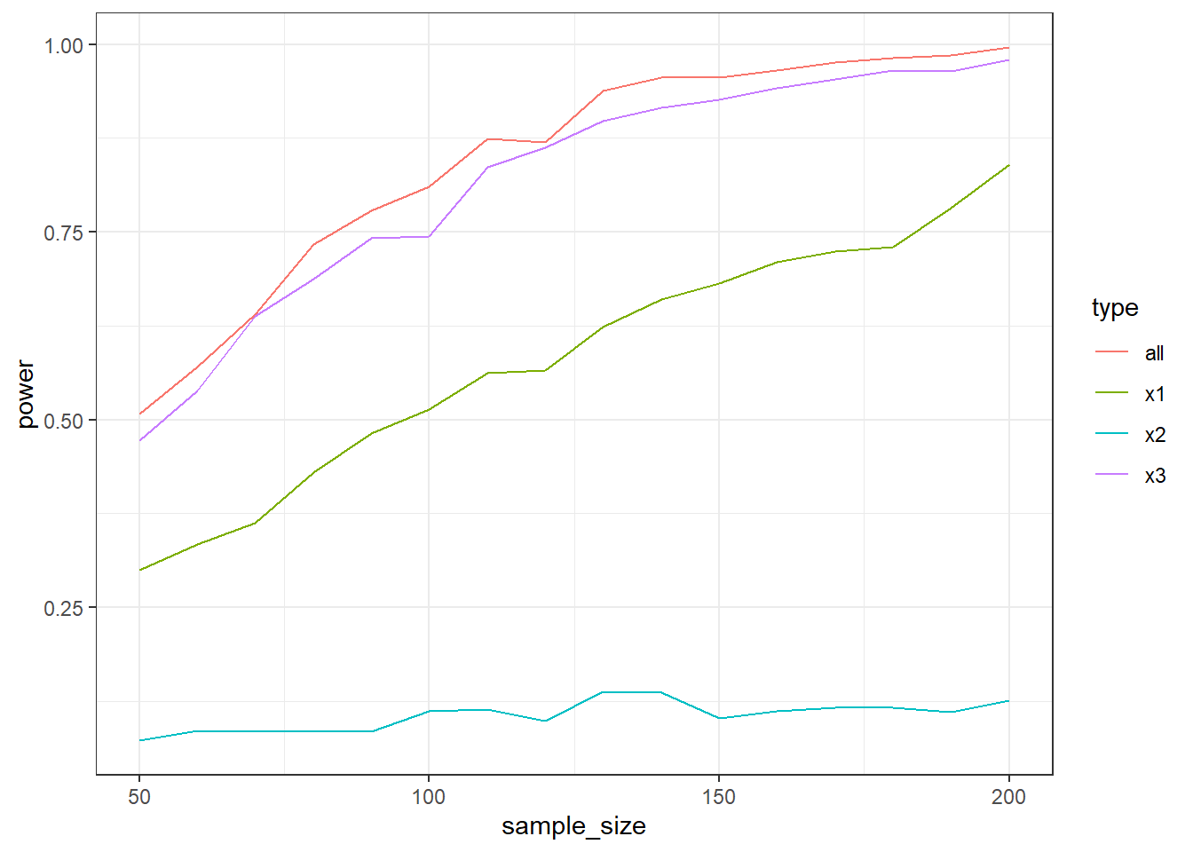
Expand to get a tip
The only new part is that you’re relying on a linear model for creating scores and that you’re storing more than one p-value from the model. Let’s declare our variables first.
b0 <- ? # outcome when all predictors are at 0
b1 <- ? # independent effect of x1
b2 <- ? # indenepdent effect of x2
b3 <- ? # independent effect of x3
sizes <- ? # the sample sizes we're iterating over
runs <- ? # number of simulations

# somewhere to store our results (type indicates which type of power estimate it is)
outcomes <-
  data.frame(
    sample_size = NULL,
    type = NULL,
    power = NULL
  )
Now we just need to fill those parameters into the linear model, put the linear model into a loop that iterates over the sample sizes, and store the results from each run.
# iterate over the sample sizes
for (? in ?) {

  # somewhere to store each type of p-value
  pvalues_all <- NULL
  pvalues_x1 <- NULL
  pvalues_x2 <- NULL
  pvalues_x3 <- NULL

  for (? in 1:?) {

    error <- ?

    x1 <- ? # uniform predictor
    x2 <- ? # uniform predictor
    x3 <- ? # uniform predictor

    # put predictors into a data frame and create the outcome score
    d <-
      data.frame(
        x1 = ?,
        x2 = ?,
        x3 = ?,
        y = ? + error
      )

    m <- summary(lm(y ~ x1 + x2 + x3, d))

    pvalues_all[?] <- broom::glance(m)$p.value
    pvalues_x1[?] <- ?
    pvalues_x2[?] <- ?
    pvalues_x3[?] <- ?
  }

  # store results somewhere
  outcomes <-
    ?
}
You’ll notice that manually creating one “container” per type of p-value isn’t great coding. It gets the job done, but in your own work, you should consider a programmatic solution.
0.2 Exercise
Create a correlation between two variables of 0.2. Use a correlation matrix. How many participants do you need for 95% power with an alpha of 0.01? Go about this as you think is best. Verify your estimate with GPower.
library(MASS)

sigma <-
  matrix(
    c(1, 0.2, 0.2, 1),
    ncol = 2
  )
alpha <- 0.01
power <- 0
n <- 100
runs <- 1e3

outcomes <-
  data.frame(
    sample_size = NULL,
    power = NULL
  )

while (power < 0.95) {

  pvalues <- NULL

  for (i in 1:runs) {

    d <-
      mvrnorm(
        n,
        c(0,0),
        sigma
      )

    d <- as.data.frame(d)

    colnames(d) <- c("x1", "x2")

    pvalues[i] <- cor.test(d$x1, d$x2)$p.value
  }

  power <- sum(pvalues < alpha) / length(pvalues)

  outcomes <-
    rbind(
      outcomes,
      data.frame(
        sample_size = n,
        power = power
      )
    )

  n <- n + 10
}

plot(outcomes$sample_size, outcomes$power)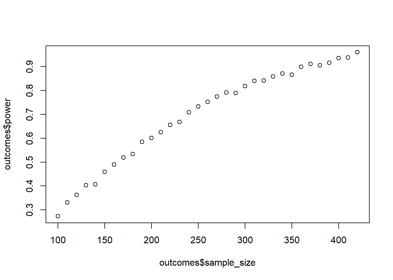
Expand to get a tip
You’re creating correlated scores, so it’s probably most straight forward to draw from a multivariate distribution. For that, we need a correlation matrix (aka a variance-covariance matrix with 0s and \(r\)s). So how will we get that matrix? Well, all we need, really, is the correlation because we already know the variance is 1:
sigma <-
  matrix(
    c(1, 0.2, 0.2, 1),
    ncol = 2
  )
Then we can get a sample as always:
d <-
  mvrnorm(
    n,
    c(0,0), # our means are 0 because the "variables" are standardized
    sigma
  )
Now you can put that into a for loop or while statement, and voila. For getting the p-value for the correlation, look at ?cor.test and inspect the object.
0.3 Exercise
In the correlation matrix, you specifically say how variables are related, but also when they aren’t related (i.e., when you assign zero for a correlation). For the data generating process, this is important, because it specifies the causal structure. Going simply by \(R^2\) or significance will often be misleading. For example, what if you have a third variable that creates a spurious effect? You can simulate that as well. Say you measure how much ice cream a person consumes in a year and expect that eating a lot of sweet, sweet ice cream makes people crave savory foods, which you measure as the portions of fries consumed in a beer garden. However, there truly is no effect of ice cream on eating fries; it’s just that both are influenced by the number of sun hours: More sun hours will lead people to eat more ice cream but also to spend more time in beer gardens and, inevitably, eat fries there.
Simulate that: Use a sample size of 10,000. First, create a sun hours variable (rnorm will be enough). Then, have sun hours cause ice cream eating with an effect size of your choosing (don’t forget some error) . Next, also have sun hours cause fries eating. Now run two regression models:
- one where you predict fries with ice cream alone
- one where you predict fries with ice cream and sun hours
Which model gives you the correct causal effect of ice cream eating? But which one has a lower p-value for the ice cream variables? Do you see how it makes little sense to just go for significance and how you must consider the causal process when simulating data? If this tickled your interest, have a look here and here.
n <- 1e4

sun <- rnorm(n)
ice_cream <- 0.4*sun + rnorm(n)
fries <- 0.5*sun + rnorm(n)

summary(lm(fries ~ ice_cream))
Call:
lm(formula = fries ~ ice_cream)

Residuals:
    Min      1Q  Median      3Q     Max
-3.8340 -0.7412 -0.0039  0.7345  4.3659

Coefficients:
            Estimate Std. Error t value Pr(>|t|)
(Intercept) 0.009393   0.011036   0.851    0.395
ice_cream   0.175206   0.010235  17.118   <2e-16 ***
---
Signif. codes:  0 '***' 0.001 '**' 0.01 '*' 0.05 '.' 0.1 ' ' 1

Residual standard error: 1.104 on 9998 degrees of freedom
Multiple R-squared:  0.02847,   Adjusted R-squared:  0.02838
F-statistic: 293 on 1 and 9998 DF, p-value: < 2.2e-16summary(lm(fries ~ ice_cream + sun))
Call:
lm(formula = fries ~ ice_cream + sun)

Residuals:
    Min      1Q  Median      3Q     Max
-3.6994 -0.6739 -0.0083  0.6723  3.6741

Coefficients:
             Estimate Std. Error t value Pr(>|t|)
(Intercept)  0.004700   0.010029   0.469    0.639
ice_cream   -0.003296   0.010080  -0.327    0.744
sun          0.497472   0.010829  45.937   <2e-16 ***
---
Signif. codes:  0 '***' 0.001 '**' 0.01 '*' 0.05 '.' 0.1 ' ' 1

Residual standard error: 1.003 on 9997 degrees of freedom
Multiple R-squared:  0.1978,    Adjusted R-squared:  0.1976
F-statistic:  1233 on 2 and 9997 DF,  p-value: < 2.2e-16
Expand to get a tip
No need to overthink this. Just follow the instructions closely. This is more of a conceptual exercise:
n <- ? # sample size

sun <- rnorm(n) # yup, that's all it takes here; we don't care about the actual values
ice_cream <- ?*sun + rnorm(n) # just put in a number; that's it
fries <- ? # same here

summary(lm(fries ~ ice_cream))
summary(lm(fries ~ ice_cream + sun))
0.4 Exercise
Your colleague comes to you and tells you that they predicted satisfaction with a film with people’s enjoyment: The higher the enjoyment, the more they reported to be satisfied with the film. However, they only had 20 people in their sample. Run a sensitivity analysis and check for what \(r\) 20 people give you 90% power, even if you allow a more liberal alpha of 0.10. Increase \(r\) in steps of 0.01 and go the full distance, checking all effect sizes from 0 to 1. Do 500 runs per step. Verify with GPower.
n <- 20
alpha <- 0.10
effects <- seq(0, 1, 0.01)
runs <- 1e3

outcomes <-
  data.frame(
    effect_size = NULL,
    power = NULL
  )

pvalues <- NULL

for (anr in effects) {

  for (i in 1:runs) {
    sigma <- matrix(
        c(1, anr, anr, 1),
        ncol = 2
      )

      d <- mvrnorm(
        n,
        c(0,0),
        sigma
      )

      d <- as.data.frame(d)
      colnames(d) <- c("enjoyment", "satisfaction")

      pvalues[i] <- cor.test(d$enjoyment, d$satisfaction)$p.value
  }

  outcomes <-
    rbind(
      outcomes,
      data.frame(
        effect_size = anr,
        power = sum(pvalues < alpha) / length(pvalues)
      )
    )
}

plot(outcomes$effect_size, outcomes$power)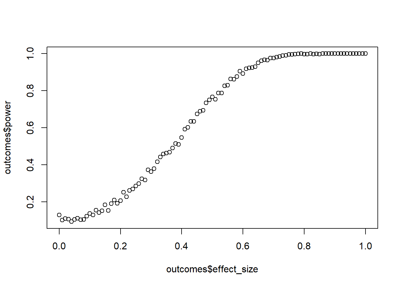
Expand to get a tip
Think back about sensitivity analysis. Here, we don’t iterate over sample sizes; we iterate over effect sizes. Because the effect size is on the standardized scale, we’ll use a correlation matrix to generate the data. The \(r\) will go into that correlation matrix, so we’ll need to create a correlation matrix for each iteration of effect size, then get a sample, run a test, and calculate power.
Let’s start with declaring our variables:
n <- ? # sample size
alpha <- ? # the alpha
effects <- seq(?, ?, 0.01) # create all rs between 0 and 1
runs <- ? # how many runs

# somewhere to store the outcome
outcomes <-
  data.frame(
    effect_size = NULL,
    power = NULL
  )
Alright, now let’s iterate over effect sizes:
for (? in ?) { # for an r in our vector of effect sizes

  for (i in 1:runs) {

    sigma <- matrix(
        c(1, ?, ?, 1), # here, we need the correlation (aka effect size) per run
        ncol = 2
      )

    # create a data frame
      d <- mvrnorm(
        ?,
        ?,
        sigma
      )

    # run cor.test and store p-value
  }

  outcomes <-
    ?
}
0.5 Exercise
You design a follow-up study where you measure enjoyment and satisfaction with films, but this time you want to determine a SESOI and do a power analysis before-hand. You measure both variables on a 5-point index Likert-scale (by index I mean it’s the average of several items). You know enjoyment usually scores above the midpoint; say a mean of 3.9 sounds realistic. The SD will be narrow: 0.5. For satisfaction, you expect a score below the midpoint of the scale, at 2.1, but with a larger SD of 1. Your smallest effect size of interest is 0.7 points because a previous analysis shows that this is the point where satisfaction translates to higher well-being for the day.
You want to be strict, so you set your alpha to 0.005, but at the same time, you don’t mind missing a true effect just as much, which is why you set your power goal to 85%. Run the power analysis (1000 runs per combo). Start at 50 people and go up in steps of 1 until you reach your desired power level (translation: use a while statement). Tip: Use the raw effect and SDs to get \(r\), which you then use in a variance-covariance matrix to simulate a data set for a given sample size. Verify with GPower.
goal <- 0.85
alpha <- 0.005
sesoi <- 0.7
n <- 50
means <- c(enjoyment = 3.9, satisfaction = 2.1)
sd_enjoy <- 0.5
sd_sat <- 1
r <- sesoi * sd_enjoy/sd_sat
covariance <- r * sd_enjoy * sd_sat
runs <- 1e3

sigma <-
  matrix(
    c(
      sd_enjoy**2, covariance,
      covariance, sd_sat**2
    ),
    ncol = 2
  )

outcomes <-
  data.frame(
    sample_size = NULL,
    power = NULL
  )

power <- 0

while (power < goal) {

  pvalues <- NULL

  for (i in 1:runs) {

    d <- as.data.frame(
      mvrnorm(
        n,
        means,
        sigma
      )
    )

    pvalues[i] <- cor.test(d$enjoyment, d$satisfaction)$p.value
  }

  power <- sum(pvalues < alpha) / length(pvalues)

  outcomes <- rbind(
    outcomes,
    data.frame(
      sample_size = n,
      power = power
    )
  )

  n <- n + 1
}

plot(outcomes$sample_size, outcomes$power)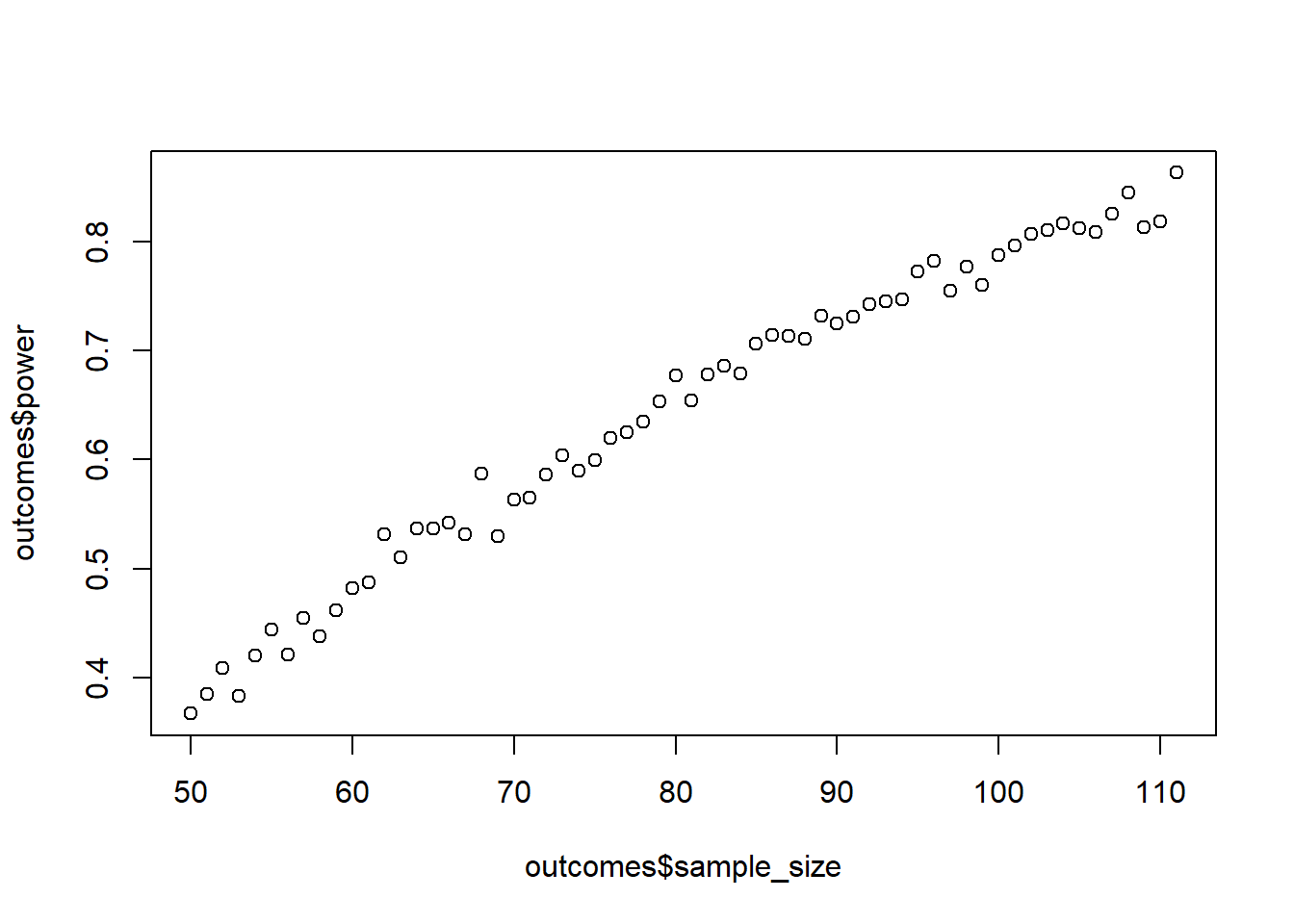
Expand to get a tip
As always, declaring our variables is a good starting point:
goal <- 0.85 # our goal for power
alpha <- ? # our stringent alpha
sesoi <- ? # what's the smallest effect size we care about?
n <- ? # what's our starting sample size?
means <- c(enjoyment = ?, satisfaction = ?)
sd_enjoy <- ? # SD of enjoyment
sd_sat <- ? # SD of satisfaction
r <- ? # what's our sesoi on the standardized scale? use the SDs of the two variables
covariance <- ? # calculate the covariance with the correlation (from the previous line) and multiply by the two SDs
runs <- 1e3
Once we have those variables, it’s a standard while statement that we’ve also done in the previous exercises.
power <- 0 # starting value for power

while (power < ?) { # keep going as long as power is below our goal (wink, wink)

  # somewhere to store our p-values

  # then we do our 1,000 simulations
  for (i in 1:?) {

    # create data frame with mvrnorm
    d <- ?

    # get your p-value from the correlation
    ? <- ?
  }

  # calculate power so that the while statement can check whether we reached our goal
  power <- ?

  # store it all somewhere

  # update something so that the power increases with each iteration
}
0.6 Exercise
A colleague has found that films with higher ratings on IMDB bring in more money at the box office. However, you think this effect is mostly due to genre: for comedies, there is an effect of quality on success, but for action films this doesn’t matter. In other words, you predict an interaction, such that the positive effect of quality (i.e., IMDB rating) is only present in one condition (genre: comedies), but not in the other condition.
You want to test that hypothesis and start your power simulation. Specifically, you want to power for the interaction effect. IMDB ratings range from 0-10. Success is measured in million dollar steps. For genre, action films will be your baseline. You’ll also center the rating so that 0 represents an average rating. Overall, when a film is an action flick and has an average rating, you expect it to bring in 20 million. You don’t expect a main effect of quality because the quality effect will depend on genre. You do expect, however, a main effect of genre, such that, at average quality, comedies bring in 5 million more than action flicks. Crucially, you expect an interaction effect: For comedies, each 1-point increase in quality will generate 2 million extra at the box office.
As for error: You expect a normally distributed error with a mean of 0 and an SD of 15. Simulate the data and see how many films you need to have enough power to detect the interaction effect with 95% power with an alpha of 0.05. Start at 10 and go up in steps of 10 to a maximum of 250. Do 1,000 runs per combo.
Like before, when you work with the linear model, it will help write out the model. So maybe start with the formula below:
\[\begin{align} millions = \beta_0 + \beta_1 Quality + \beta_2 Genre + \beta_3 Quality \times Genre + \epsilon \end{align}\]First start by filling in the betas and using them to simulate a massive data set (say 10,000 cases) before you start simulating. Plot the data set with:
ggplot(d, aes(x = quality, y = success, color = genre)) +
  geom_point(alpha = 0.5) +
  geom_smooth(method = "lm") +
  theme_bw()
Does the plot look like what we specified? Make sure you code the factor correctly: genre should have action films as the baseline; otherwise, the meaning of \(\beta_2\) and \(\beta_3\) changes.
b0 <- 50
b1 <- 0
b2 <- 5
b3 <- 2
sizes <- seq(10, 300, 10)
runs <- 1e3

outcomes <-
  data.frame(
    sample_size = NULL,
    power = NULL
  )

for (n in sizes) {

  pvalues <- NULL

  for (i in 1:runs) {

    error <- rnorm(n, 0, 15)
    genre <-  rep(0:1, n/2)
    quality <-  scale(runif(n, 0, 10), center = TRUE, scale = FALSE)

    d <-
      data.frame(
        genre = genre,
        quality = quality,
        success = b0 + b1*quality + b2*genre + b3*quality*genre + error
      )

    # success can't be less than 0
    d$success <- ifelse(d$success < 0, 0, d$success)

    m <- summary(lm(success ~ quality*genre, d))

    pvalues[i] <- broom::tidy(m)$p.value[4]

  }

  outcomes <-
    rbind(
      outcomes,
      data.frame(
        sample_size = n,
        power = sum(pvalues < 0.05) / length(pvalues)
      )
    )
}

with(outcomes, plot(sample_size, power))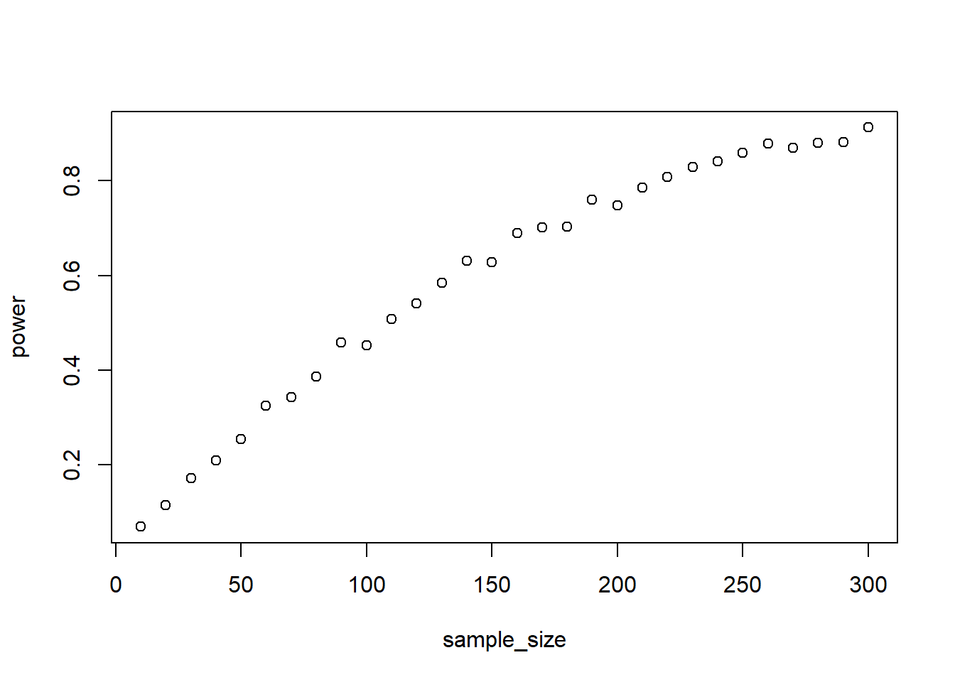
Expand to get a tip
We need to fill in the betas for the linear model formula, so let’s define them:
b0 <- ? # action flick at average quality
b1 <- ? # main effect quality: going 1 up on quality for action films
b2 <- ? # main effect genre: going from action to comedy at average quality
b3 <- ? # the extra information when being a comedy and increasing in quality
sizes <- seq(?, ?, ?)
runs <- 1e3
After that, we can simply run a loop. Just remember to create “fresh” error per run and not define it as a constant with the other parameters above.
for (? in ?) {

  pvalues <- NULL

  for (i in 1:?) {

    error <- ?
    genre <-  rep(0:1, ?)
    quality <-  runif(?, ?, ?)
    # don't forget to center

    d <-
      data.frame(
        genre = ?,
        quality = ?,
        success = b0 + b1*? + b2*? + b3*?*? + ?
      )

    # success can't be less than 0

    # get p-value for interaction

  }
}
0.7 Exercise
Simulate the above again, but this time increase the main effects of both quality and genre to 10 million. Leave the interaction effect at 2. What do you think – will this have an effect on power? If so, how and why?
b0 <- 50
b1 <- 10
b2 <- 10
b3 <- 2
sizes <- seq(10, 250, 10)
runs <- 1e3

outcomes <-
  data.frame(
    sample_size = NULL,
    power = NULL
  )

for (n in sizes) {

  pvalues <- NULL

  for (i in 1:runs) {

    error <- rnorm(n, 0, 15)
    genre <-  rep(0:1, n/2)
    quality <-  scale(runif(n, 0, 10), center = TRUE, scale = FALSE)

    d <-
      data.frame(
        genre = genre,
        quality = quality,
        success = b0 + b1*quality + b2*genre + b3*quality*genre + error
      )

    # success can't be less than 0
    d$success <- ifelse(d$success < 0, 0, d$success)

    m <- summary(lm(success ~ quality*genre, d))

    pvalues[i] <- broom::tidy(m)$p.value[4]

  }

  outcomes <-
    rbind(
      outcomes,
      data.frame(
        sample_size = n,
        power = sum(pvalues < 0.05) / length(pvalues)
      )
    )
}

with(outcomes, plot(sample_size, power))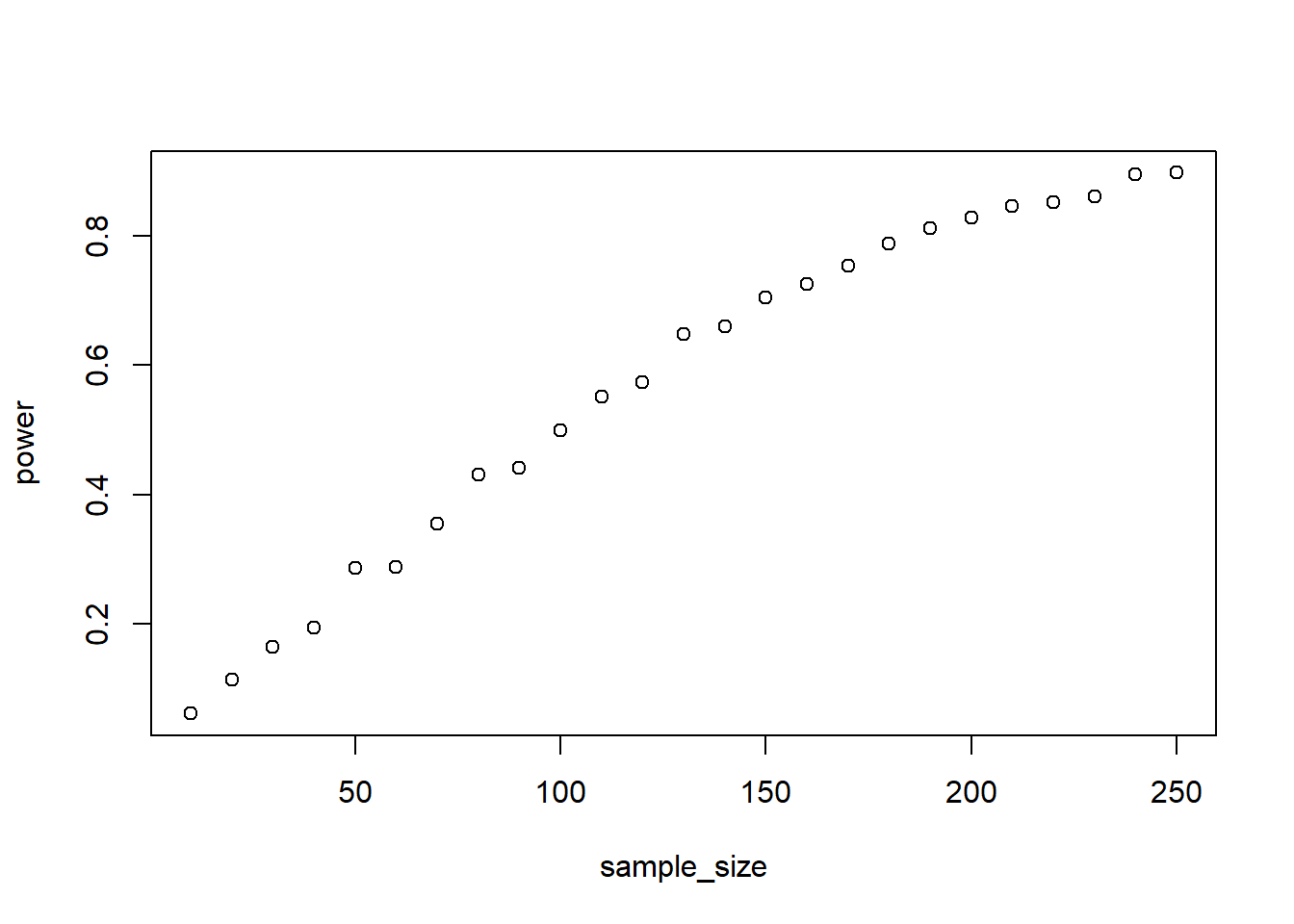
0.8 Exercise
You want to know how much listening to music leads to feelings of being relaxed. You expect a linear effect of the number of songs someone listens to on them feeling relaxed. After all, if listening to music relaxes you, then the more music, the more relaxed you get.
However, you suspect that whether this effect occurs will strongly depend on how much people like these songs. Can’t relax if you listen to lots of crap (notice how I didn’t mention an artist here to be nice).
You measure feelings of relaxation on a Likert-type index variable with a range of 1-7. The number of songs is measured as a count with a maximum of 30 songs–you counted songs over a 1h period. After that period, you also asked how much people enjoyed the songs they were listening to on a scale from 0-100.
Simulate number of songs (use sample) and liking (uniform). Transform the number of songs so that 1 up on the variable means listening to 5 more songs. As for liking, you want to go in steps of 10. Center both. These transformations make it easier to get an intuition about the effect sizes.
At average listening and liking, you think relaxation should be somewhat below the midpoint of the scale: 3.1. You don’t expect main effects of either predictor: Liking music shouldn’t relax you unless you listen to some of it, and listening to music alone shouldn’t do much unless you like the music.
However, you expect a fairly sizable interaction effect, such that the combination of liking and listening will increase relaxation by 0.2 points. Remember the transformations: We say that listening to 5 songs (which is going up 1 on the listening variable) will increase relaxation 0.2 when liking also goes up by 10 points (which is going up 1 on the liking variable).
For error, you expect a normally distributed error with mean 0 and an SD of 2. Simulate power for the interaction effect, starting at 10 and ending at a sample size of 100. Go in steps of 5.Do 1,000 runs per combo. Also use interactions::interaction_plot to plot a random model to check how the data look like.
b0 <- 3.1
b1 <- 0
b2 <- 0
b3 <- 0.2
sizes <- seq(10, 100, 5)
runs <- 1e3

outcomes <-
  data.frame(
    sample_size = NULL,
    power = NULL
  )

for (n in sizes) {

  pvalues <- NULL

  for (i in 1:runs) {

    error <- rnorm(n, 0, 2)
    listening <- scale(sample(1:30, n, replace = TRUE) / 5, scale = FALSE)
    liking <- scale(runif(n, 0, 100) / 10, scale = FALSE)

    d <-
      data.frame(
        listening = listening,
        liking = liking,
        relaxation = b0 + b1*listening + b2*liking + b3*listening*liking + error
      )

    #trim the outcome
    d$relaxation <- ifelse(d$relaxation < 0, 0, d$relaxation)
    d$relaxation <- ifelse(d$relaxation > 7, 7, d$relaxation)

    m <- summary(lm(relaxation ~ listening*liking, d))
    pvalues[i] <- broom::tidy(m)$p.value[4]
  }

  outcomes <-
    rbind(
      outcomes,
      data.frame(
        sample_size = n,
        power = sum(pvalues < 0.05) / length(pvalues)
      )
    )

}

plot(outcomes$sample_size, outcomes$power)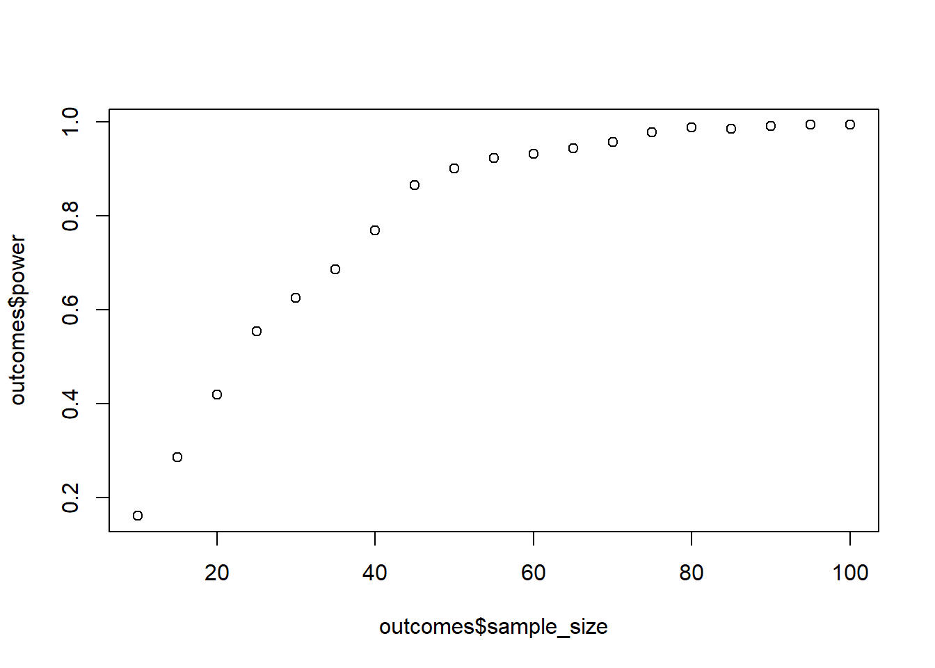
interactions::interact_plot(lm(relaxation ~ listening*liking, d), pred = "listening", modx = "liking")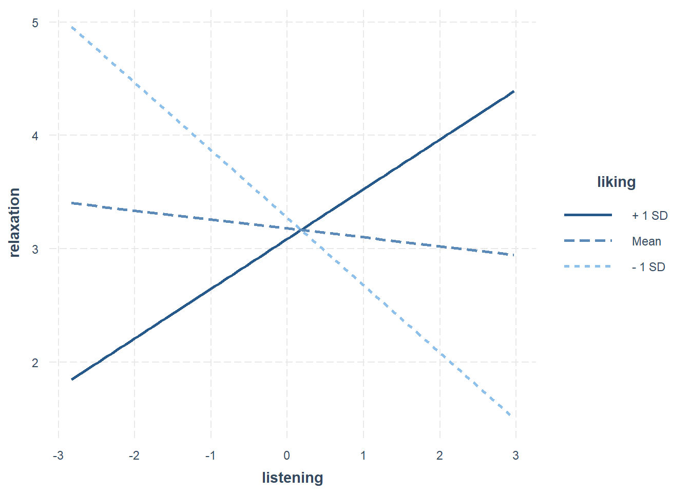
Expand to get a tip
The actual work here is thinking through correctly defining and transforming the variables. So let’s declare first, then think about the transformations.
b0 <- ? # relaxation when both liking and number of songs variables are at average
b1 <- ? # main effect listening: going up 1 on number of songs variable while liking variable is at average
b2 <- ? # main effect liking: going up 1 on liking variable whilst number of songs variable is at average
b3 <- ? # the extra information when we listen to 5 songs (= going 1 up on number of songs variable) and like them 10 points more (= going up 1 on liking variable)
sizes <- seq(?, ?, ?)
runs <- 1e3
Okay, that still doesn’t solve the transformation problem. How do we make the variables? Well, there’s 3 steps each for the listening and the liking variable:
- Get the raw variable (with
sampleorrunif) - Transform it such that 1 point on the variable now means something different
- Center this transformed variable
# gets us a uniform distribution of songs
listening <- sample(1:30, ?, replace = ?)

# easy as that: divide by 5 to change a 1-unite increase on the variable
listening <- listening / 5

# center
listening <- scale(?)
The process for liking is similar. Once you have that figured out, the rest of the steps are as known: For each simulation, create those variables and use them in the linear model to generate a relaxation score; obtain p-values; calculate power.