library(tidyverse)

twobytwo <-
  function(
    means = c(0, 0, 0, 0),
    factors = c("Factor 1", "Factor 2"),
    levels1 = c("Level 1", "Level 2"),
    levels2 = c("Level 1", "Level 2"),
    outcome = "Outcome"
  ){
    d <-
      data.frame(
        f1 = rep(levels1, times = 2),
        f2 = rep(levels2, each = 2),
        outcome = means
      )

    names(d) <- c(factors, outcome)

    p <-
      ggplot(d, aes(x = .data[[factors[1]]], y = .data[[outcome]], shape = .data[[factors[2]]], group = .data[[factors[2]]])) +
      geom_point(size = 3) +
      geom_line(aes(linetype = .data[[factors[2]]]), size = 1) +
      theme_bw() +
      theme(
        axis.ticks.y = element_blank(),
        axis.text.y = element_blank()
      )

    return(p)
}Exercise V
Overview
In this set of exercises, you’ll test your understanding of interactions. You’ll start with simulating power for an interaction, before going into more detail of what that actually means. You play around with different effect sizes (and ways to approach interactions) to find out how that affects power. Please note: All experiments and previous research below are completely fictional–not like I have any idea what I’m talking about.
0.1 Exercise
You plan to analyze data from a content analysis. You’re interested in what predicts the number of Twitter followers for celebrities (including C-list celebrities, whatever that means). You believe that blue check mark definitely means having more followers compared to not having a check mark. Your dependent measure is, well, just the number of followers. You also expect that this difference will be stronger if a celebrity is more active, say tweets at least once a week.
Now you want to run a power analysis to test that idea. First draw (on a piece of paper or digitally) your interaction. You can use the function below to try out some “drawings”. Start with putting in some of the means to roughly get the pattern described above.
For example, the below would be a complete reversal:
twobytwo(
  means = c(0, 2, 2, 0),
  factors = c("Verified", "Activity"),
  levels1 = c("No", "Yes"),
  levels2 = c("Lurker", "Active"),
  outcome = "Followers"
)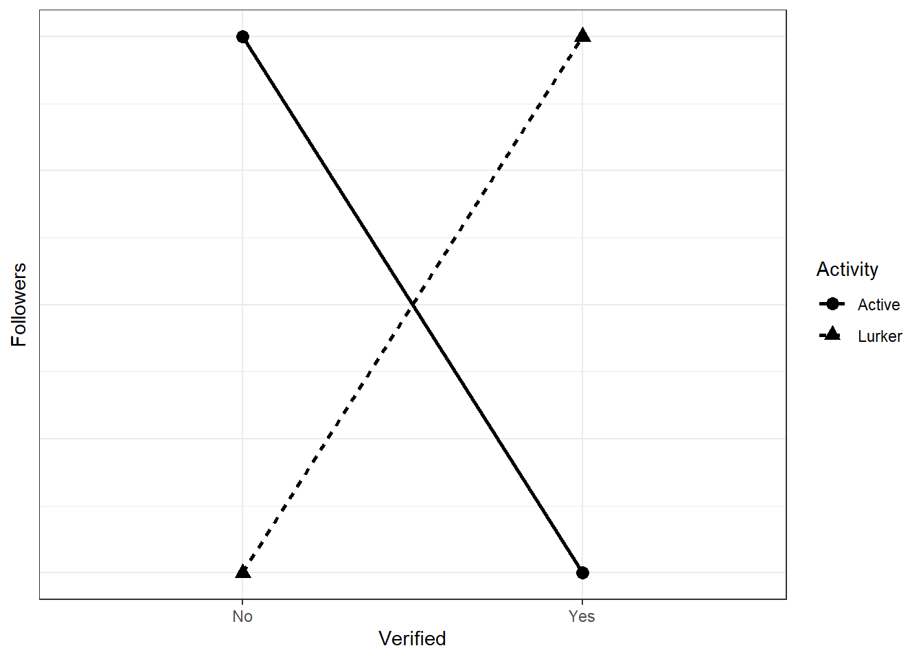
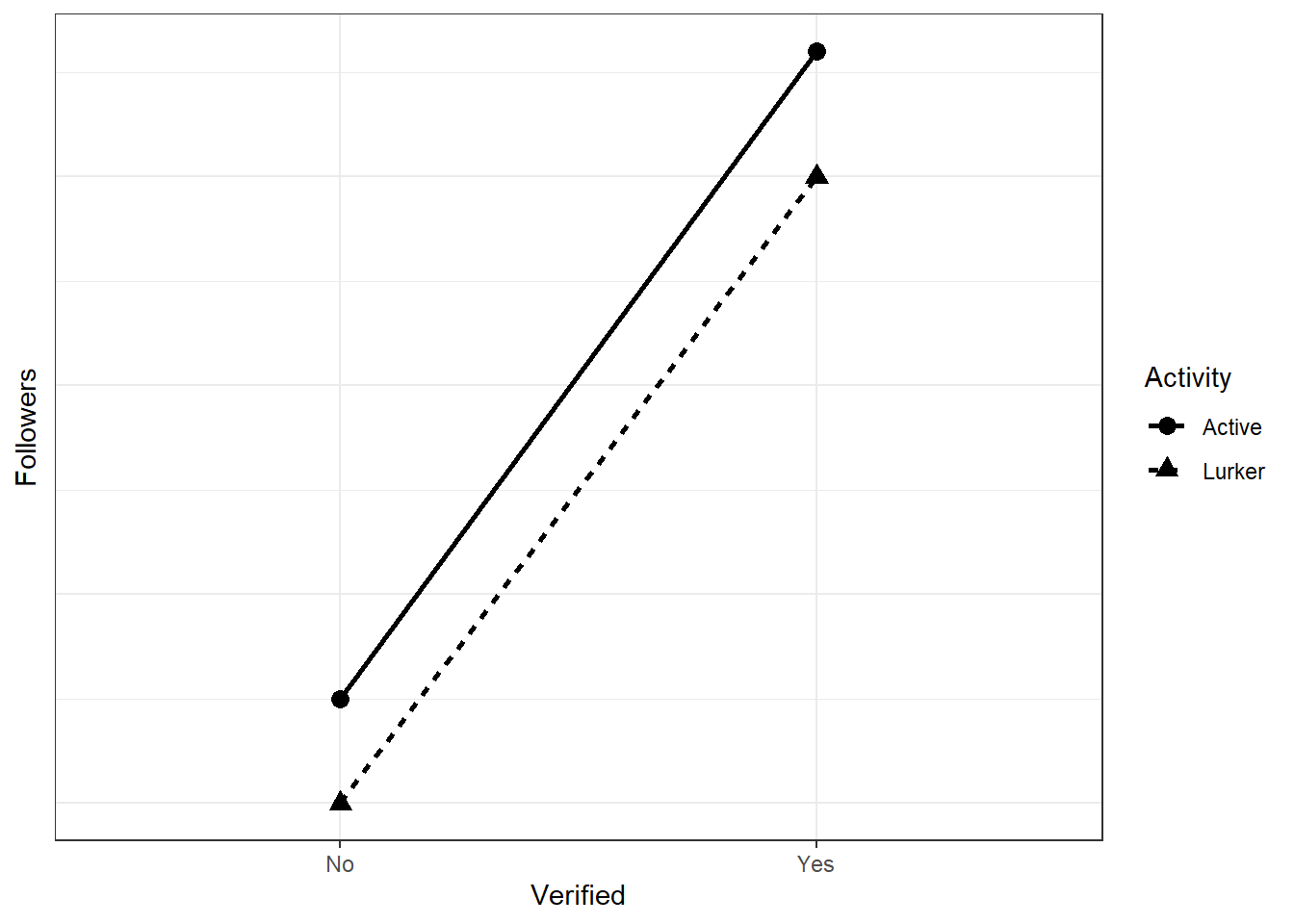
For our case, we’re interested in an attenuation effect: There’s an effect of verification (well, it’s not a causal effect in that sense, but let’s not get into that for now) regardless of the activity type, but it’ll be stronger with higher activity. How much stronger? And what follower counts should you expect for the different groups? This is where common sense and thinking about effect sizes on the raw scale comes in. Let’s go back to the linear model:
\(Characters = \beta_0 + \beta_1Verification + \beta_2Activity + \beta_3Verification \times Activity + \epsilon\)
Go back to the slides if you need a refresher what each beta represents. Let’s talk about our expectations. Let’s say we expect those without verification and low activity to have something like 20,000 followers. We expect that verification makes a big difference, such that verified celebrities, even when they’re not active, have, on average, 50,000 followers. Now comes the tricky bit: How many more followers will an unverified, but active person have? Let’s say it’s 25,000. As for the interaction: How much does activity add to the already massive difference between unverified and verified lurkers? Let’s say it adds 1,000 followers.
Run a power analysis with these values where you figure out how many participants you need per group. “Recruiting” people won’t be difficult, so all you need is a rough estimate. Start at 500 celebrities and then go up in steps of 20 until 1,500. Use the linear model from above to create the scores. As for error: You’re really not sure about your estimates, so you add a lot of error. Use a normally distributed error term of 5,000 with a standard deviation of 5,000. For now, you’re not interested in the actual contrasts, only in whether an interaction is present. So run an lm model with and one without the interaction term and compare them with anova. Do 1,000 runs per combo. Also, you really don’t want to commit a Type I error, so you set your alpha to 0.001.
set.seed(42)

b0 <- 2e4
b1 <- 3e4
b2 <- 5e3
b3 <- 1e3
sizes <- seq(500, 1500, 20)
runs <- 1e3

outcomes <-
  data.frame(
    sample_size = NULL,
    power = NULL
  )

for (n in sizes) {

  pvalues <- NULL

  for (i in 1:runs) {

    d <-
      data.frame(
        Verification = rep(0:1, times = n*2),
        Activity = rep(0:1, each = n*2)
      )

    d$Followers <- b0 + b1*d$Verification + b2*d$Activity + b3*d$Verification*d$Activity + rnorm(n, 5e3, 5e3)

    mains <- lm(Followers ~ Verification + Activity, d)
    interactions <- lm(Followers ~ Verification*Activity, d)

    pvalues[i] <- anova(mains, interactions)$`Pr(>F)`[2]
  }

  outcomes <-
    rbind(
      outcomes,
      data.frame(
        sample_size = n,
        power = sum(pvalues < .001) / length(pvalues)
      )
    )
}

plot(outcomes$sample_size, outcomes$power)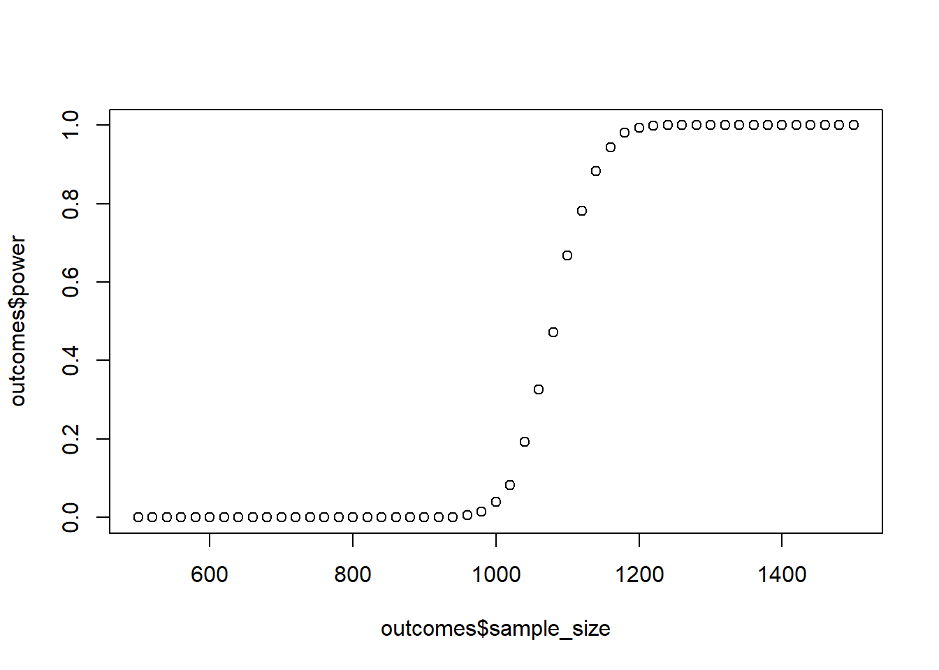
Expand to get a tip
As always, begin with declaring your variables:
b0 <- ? # unverified lurkers
b1 <- ? # verified active
b2 <- ? # unverified, but active
b3 <- ? # the extra for being both verified and active
sizes <- seq(?, ?, ?) # the steps in which we go up
runs <- ? # how many simulations per combo

# somewhere to store
outcomes <-
  data.frame(
    sample_size = NULL,
    power = NULL
  )
Alright, if we’re working with the linear model, we just need a data frame that has two variables (Activity and Verification); each one should either be 0 or 1. So you’ll need to play around with rep to get the right combination. Then, you just fill in the linear model to create a third variable that holds the number of followers. Everything after that is just doing two lm models and comparing them to obtain a p-value.
# iterate over sample sizes
for (? in ?) {

  # store p-values
  pvalues <- NULL

  for (i in 1:runs) {

    # create the data frame
    d <-
      data.frame(
        Verification = ?,
        Activity = ?
      )

    # get our dependent variable (don't forget to add error in the end)
    d$Followers <- ? + b1*? + b2*d$Activity + ?*d$Verification*? + rnorm(?, ?, ?)

    # construct the two models
    mains <- lm(? ~ ? + ?, d)
    interactions <- lm(? ~ ?, d)

    pvalues[?] <- anova(mains, interactions)$`Pr(>F)`[2]
  }

  # and store
  outcomes <-
    rbind(
      outcomes,
      data.frame(
        sample_size = n,
        power = sum(pvalues < .001) / length(pvalues)
      )
    )
}
You can plot the power curve as always with plot(outcomes$sample_size, outcomes$power).
0.2 Exercise
We conduct an experiment. Previous research has shown that reading a story in the first person leads to more enjoyment on a 7-point Likert-scale than in the third person. For your thesis, you want to understand that effect better. You believe that the effect will be stronger if there’s lots of action compared to a tame story. In fact, you think that story type can completely knock out the effect (see here): The first-person enjoyment effect will only occur with an action story, but not with a lame one.
The linear model for enjoyment, measured on a 7-point Likert-scale, is as follows:
\(Enjoyment = \beta_0 + \beta_1Perspective + \beta_2Type + \beta_3Perspective \times Type\)
You believe the \(\beta\) are as follows:
\[\begin{align} &\beta_0 = 4.3\\ &\beta_1 = 0.01\\ &\beta_2 = -0.03\\ &\beta_3 = 0.4 \end{align}\]First draw the interaction to make sure you understand what it’s supposed to look like (either on paper or digitally). \(Perspective\) is 0 = 3rd person and 1 = First person; \(Type\) is 0 = Lame and 1 = Lots of action. This time, you’d like to decompose the error, meaning rather than adding overall variance, you want to add variance per group. Therefore, you simulate the data with four group means, not with the linear model (you can work the means out with the beta weights and the linear model). You set the SD to 0.6 for all groups, except for the first-person action condition where you expect opinions will be a bit more divided, setting the SD here to 0.9.
Even though you want to power for the interaction, you’re also interested in main effects you can interpret. Therefore, use type 3 sums of squares with sum-to-zero coding for the factors (afex::aov_car will do that automatically). Start at 30 participants per group and keep going in steps of 5 per group until you reach 95% power (so use a while statement). Because this is exploratory, and you really don’t want to miss an effect, you set your alpha to 0.15. Do 1,000 runs per combo.
Tip: Be careful with factor levels. R will assign levels based on the alphabet. So assigning c("3rd person", "1st person") to a factor will make the 1st person the reference category. Verify that you have the correct means by inspecting the raw means per group (i.e., create a large data set and check the means per group are the ones you intended).
set.seed(42)

means <- c(4.3, 4.31, 4.27, 4.3+0.01-0.03+0.4)
sds <- c(rep(0.6, 3), 0.9)
alpha <- 0.15
draws <- 1e3
n <- 30

outcomes <-
  data.frame(
    sample_size = NULL,
    power = NULL
  )

power <- 0

while (power < .95) {

  power <- NULL
  pvalues <- NULL

  for (i in 1:draws) {

    d <-
      data.frame(
        id = factor(1:c(4*n)),
        Enjoyment = rnorm(n*4, means, sds),
        Perspective = factor(rep(c("3rd Person", "First Person"), times = n*2)),
        Action = factor(rep(c("Lame", "Lots of action"), times = n, each = 2))
      )

    m <- suppressMessages(afex::aov_car(Enjoyment ~ Perspective*Action + Error(id), data = d))

    pvalues[i] <- m$anova_table$`Pr(>F)`[3]
  }

  power <- sum(pvalues < alpha) / length(pvalues)

  outcomes <-
    rbind(
      outcomes,
      data.frame(
        sample_size = n,
        power = power
      )
    )

  n <- n + 5
}

plot(outcomes$sample_size, outcomes$power)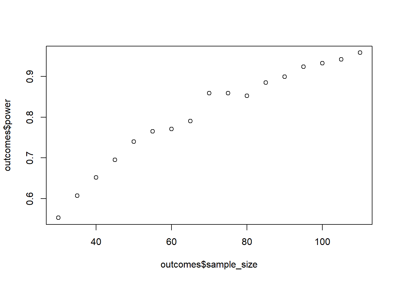
Expand to get a tip
As always, begin with declaring your variables:
means <- ? # you can get those from the betas and the linear model
sds <- ? # remember that one SD is different
alpha <- ? # we're less stringent
draws <- ? # how many runs?
n <- ? # starting sample size

# somewhere to store our data
outcomes <-
  data.frame(
    sample_size = NULL,
    power = NULL
  )
Next, we need to initiate a while loop. Within that while statement, we run 1,000 simulations for each sample size. For each, we create a data frame with an id variable, an Enjoyment variable for our outcome, as well as two variables that indicate group membership (Perspective and Action). The structure of that data frame will depend on how you create the scores for Enjoyment (if you’re completely lost, have a look at the tip for the next exercise). To be certain you’re doing things correctly, create your data set with a massive sample and verify it’s doing what it’s supposed to do (so inspect means per group, for example with aggregate(Enjoyment ~ Perspective + Action, data = d, FUN = mean)).
# initialize power

# start loop
while (power < .95) {

  # create objects to store power and p-values
  power <- NULL
  pvalues <- NULL

  for (i in 1:draws) {

    # make the score on way or the other (you could also create 4 distinct groups and then merge them)
    d <-
      data.frame(
        id = ?,
        Enjoyment = ?,
        Perspective = ?,
        Action = ?
      )

    # do the model
    m <- afex::aov_car(? ~ ?*? + Error(?), data = ?)

    pvalues[?] <- m$anova_table$`Pr(>F)`[?]
  }

  power <- ?

  outcomes <-
    ?

  # don't forget to go up a step in the sample size
}
You can plot the power curve as always with plot(outcomes$sample_size, outcomes$power).
0.3 Exercise
GPower will give you the same sample size for a power analysis for an interaction as for a t-test if the effect size of the interaction is the same as in the t-test. Let’s check that. The effect size is the same if the effect is completely reversed (see here once more). Let’s say our first experiment produced a difference between control and treatment of 15 points. The mean and SD of the control were 100 and 15. For treatment: 115 and 15. That’s a massive effect size of one standard deviation. Now would a complete reversal look like? As in: A second factor completely reverse the effect of the first factor. Like this, using the plotting function from above:
twobytwo(means = c(100, 115, 115, 100))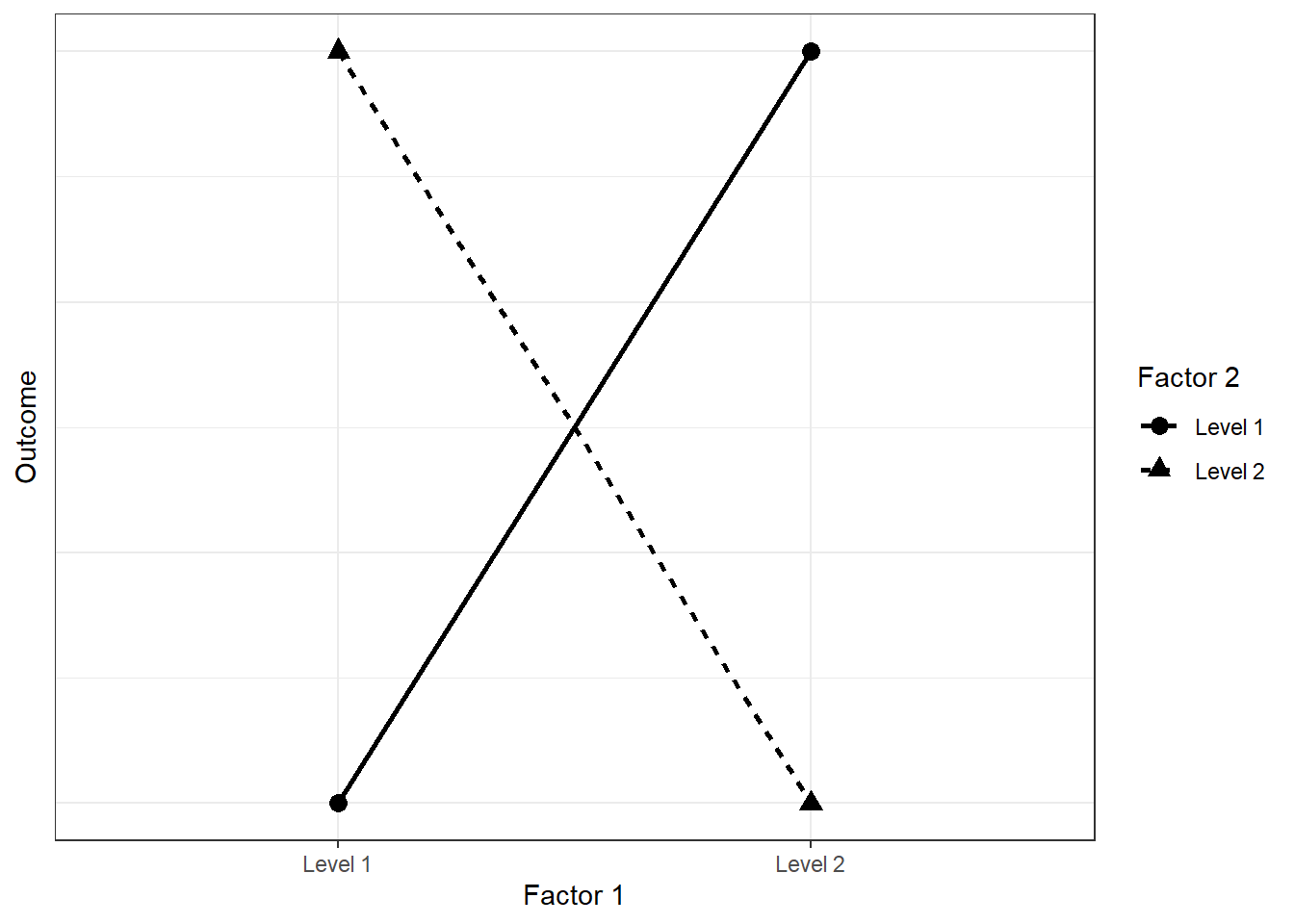
First, calculate power for the original effect (Circles above in the graph) in GPower (two-tailed). Alpha is 0.05 and power should be 95%. The groups should have the same size. Now simulate the above interaction and calculate power for the interaction effect. Compare your estimate to the GPower estimate you just got. Go about it as you think is best. (Tip: Turn the solution into a function; you’ll need it again for the next exercises.)
set.seed(42)

interaction_power <- function(
    means = c(100, 115, 115, 100),
    sd = 15,
    sizes = 1:20,
    draws = 1e3
) {
  outcomes <-
    data.frame(
      sample_size = NULL,
      power = NULL
    )

  for (n in sizes) {

    pvalues <- NULL

    for (i in 1:draws) {

      d <-
        data.frame(
          id = factor(1:c(4*n)),
          scores = rnorm(n*4, means, sd),
          factor1 = factor(rep(c("level1", "level2"), times = n*2)),
          factor2 = factor(rep(c("level1", "level2"), times = n, each = 2))
        )

      mains <- lm(scores ~ factor1 + factor2, d)
      interactions <- lm(scores ~ factor1 + factor2 + factor1:factor2, d)

      pvalues[i] <- anova(mains, interactions)$`Pr(>F)`[2]
    }

    outcomes <-
      rbind(
        outcomes,
        data.frame(
          sample_size = n,
          power = sum(pvalues < 0.05) / length(pvalues)
        )
      )
  }

  return(outcomes)
}

results <- interaction_power(draws = 200)

plot(results$sample_size, results$power)
abline(h = 0.95)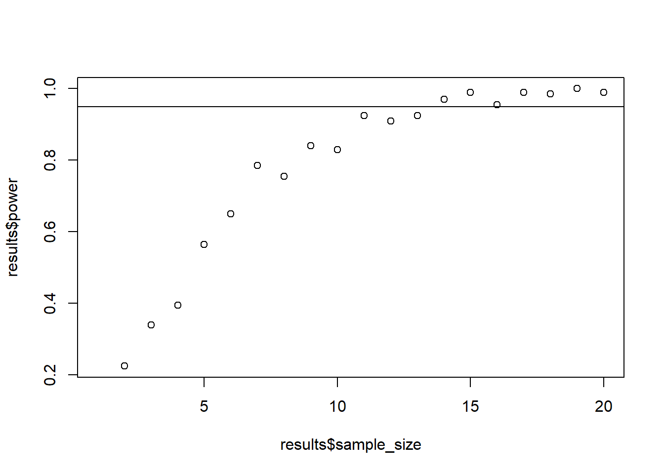
Expand to get a tip
Essentially, you can take the code from the previous exercise and put it into a function. The biggest challenge will be to make sure the groups have the “correct” means. In other words, the data frame should have the right structure. Let’s go to our means. Say we put our means into a vector: c(100, 115, 115, 100). Now when we call rnorm(n, our_means), it will go one case for 100, one for 115, one for 115, one for 100, and then repeat (remember vectorization). That means our factors in the data frame should have the following structure:
  id factor1 factor2 means
1  1  level1  level1   100
2  2  level2  level1   115
3  3  level1  level2   115
4  4  level2  level2   100
0.4 Exercise
What if an effect is attenuated? Say the original effect was between two groups with means of 4.4 and 4.9 and SDs of 0.6 and 0.7, respectively. Calculate Cohen’s d, then put that into GPower for an independent t-test (two-tailed) with an alpha of 0.05. Note down the sample size needed for 95% power. Next, we introduce a second factor that attenuates the original effect, such that the effect is half as large when we consider the second condition. The graph below (hopefully) shows what I mean:
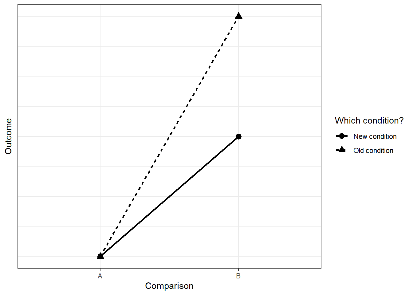
That means for the two groups under the new condition, we need to half the effect size. First, half the effect size that you put into GPower and calculate the sample size again. Note down the number you get. Then get to simulation: For the new (half-sized) two groups, half the difference between them. The SDs can be the same as for the first two groups. Calculate power for the interaction effect and compare the sample size needed for 95% to the two estimates you got from GPower. To save yourself time, use the function you wrote for the previous exercise. Also, use the GPower estimates as a ballpark figure to set your sample sizes in the simulation. What does adding an interaction add to your sample size? Compare to the case here. Tip: You’ll need to calculate the standardized effect size first for GPower; then set the means for the new two groups in relation to that standardized effect size.
So first you calculate the pooled SD for the original group; with that, you can get Cohen’s \(d\) for the original effect. Next, you can use the original means plus half a Cohen’s \(d\) (so Cohen’s \(d\) times half a pooled SD).
set.seed(42)

m1 <- 4.4
m2 <- 4.9
sd1 <- 0.6
sd2 <- 0.7
pooled_sd <- sqrt((sd1**2 + sd2**2)/2)
d <- (m2-m1)/pooled_sd

means <- c(m1, m2, m1, m1 + d/2*pooled_sd)

results <- interaction_power(
  means = means,
  sd = rep(c(sd1, sd2), 2),
  sizes = seq(100, 800, 50),
  draws = 1e3
)

plot(results$sample_size, results$power)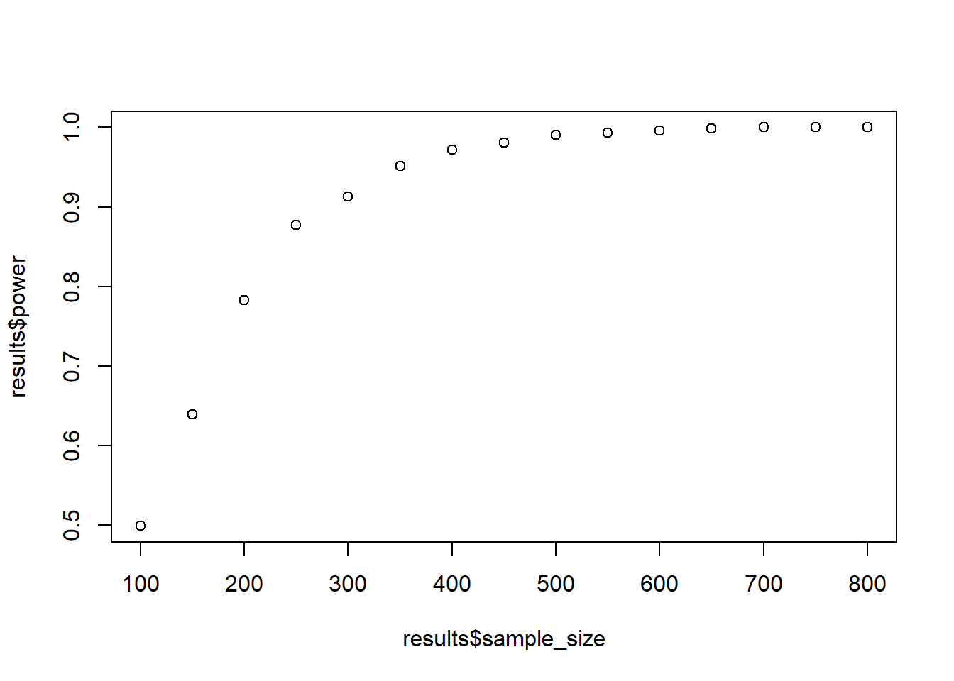
Expand to get a tip
Let’s first declare our variables:
m1 <- 4.4
m2 <- 4.9
sd1 <- 0.6
sd2 <- 0.7
pooled_sd <- ?
d <- (m2-m1)/pooled_sd
Now we know the means for the first two groups: c(4.4, 4.9). For the next two groups under the new condition, the first mean can stay the same: 4.4. All we need is a mean that’s half the size of the previous difference in pooled SD units: c(m1, m2, m1, m1 + d/2*pooled_sd).
Now you can easily feed these means to the function you wrote above.
0.5 Exercise
So far, we’ve only considered the overall interaction effect. But a significant interaction can mean many different patterns, which is why we always follow up with simple effects. Take the attenuation from the previous exercise: There are 6 comparisons that could be of interest to us, one for each possible contrast. Say for our hypothesis of attenuation to hold, we’re interested in two simple effects: The comparison of the two levels under the old condition and the comparison of the two levels under the new condition.
Therefore, repeat the above simulation, but this time also extract the p-values of these two posthoc simple effects. You can do that with pairs(emmeans::emmeans(interactions, "factor1", by = "factor2")). Save the power of the overall interaction term and the two simple effects and plot them. You can use the following code, assuming your data frame is called results, has a variable with the sample size sample_size, the type of power type, and power. You’ll need to adjust your function above or start from scratch. What’s the power of the simple effects compared to the overall interaction effect?
library(ggplot2)

ggplot(results, aes(x = sample_size, y = power, color = type, group = type)) + geom_point() + theme_bw()set.seed(42)
interaction_power <- function(
means = c(4.4, 4.9, 4.4, 4.65),
sd = rep(c(sd1, sd2), 2),
sizes = seq(50, 600, 50),
draws = 1e3
) {
outcomes <-
  data.frame(
    sample_size = NULL,
    type = NULL,
    power = NULL
  )
for (n in sizes) {
pvalues <- NULL
pvalues_simple1 <- NULL
pvalues_simple2 <- NULL
for (i in 1:draws) {
d <-
data.frame(
id = factor(1:c(4*n)),
scores = rnorm(n*4, means, sd),
factor1 = factor(rep(c("level1", "level2"), times = n*2)),
factor2 = factor(rep(c("level1", "level2"), times = n, each = 2))
)
mains <- lm(scores ~ factor1 + factor2, d)
interactions <- lm(scores ~ factor1 + factor2 + factor1:factor2, d)
ps <- data.frame(pairs(emmeans::emmeans(interactions, "factor1", by = "factor2")))
pvalues[i] <- anova(mains, interactions)$`Pr(>F)`[2]
pvalues_simple1[i] <- ps$p.value[1]
pvalues_simple2[i] <- ps$p.value[2]
}
outcomes <-
rbind(
outcomes,
data.frame(
sample_size = rep(n, 3),
type = factor(c("interaction", "simple full", "simple half")),
power = c(
sum(pvalues < 0.05) / length(pvalues),
sum(pvalues_simple1 < 0.05) / length(pvalues_simple1),
sum(pvalues_simple2 < 0.05) / length(pvalues_simple2)
)
)
)
}
return(outcomes)
}
results <- interaction_power(draws = 500)
library(ggplot2)
ggplot(results, aes(x = sample_size, y = power, color = type, group = type)) + geom_point() + theme_bw()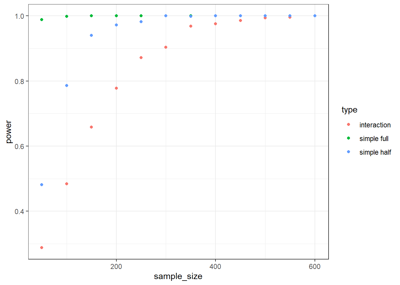
Expand to get a tip
We can take the function code from above and update it. Essentially, all we need it two more numbers per simulation: the p-value for the first contrast and the p-value for the second contrast. Out storage data frame looks as follow:
outcomes <-
data.frame(
sample_size = NULL,
type = NULL,
power = NULL
)Next, we need to access the p-values from the posthoc comparisons. So it’s best we store them with data.frame(pairs(emmeans::emmeans(interactions, "factor1", by = "factor2"))). Once we have that stored in an object, we can access the two p-values with the dollar sign and indexing ($p.value[1]). All that’s left to do is to save them all into our outcomes data frame:
outcomes <-
  rbind(
    outcomes,
    data.frame(
      sample_size = rep(n, 3),
      type = factor(c("interaction", "simple full", "simple half")),
      power = c(
        sum(pvalues < 0.05) / length(pvalues),
        sum(? < 0.05) / length(?),
        sum(? < 0.05) / length(?)
      )
    )
  )
0.6 Exercise
You want to know what leads people to change their opinion about an issue. Previous research shows that the amount of arguments leads to stronger persuasiveness of a message. That effect will be knocked out, you believe, if the message comes from a source with low credibility. Therefore, you expect something like this:
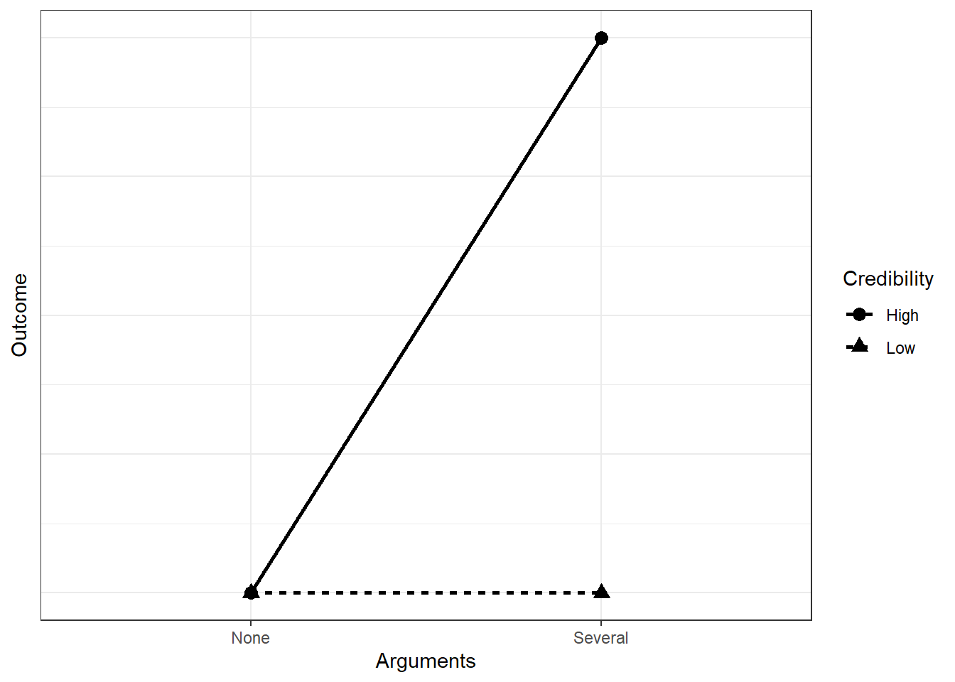
You go for a repeated measures design, where people read four stories, one in each condition, and report how persuasive they find the story to be. (For the sake of argument, let’s ignore order or carry-over effects). You measure the outcome on a 100-point scale. Without knowing any better, you assume the no arguments, low credibility condition will fall on the middle of the scale. That makes it easy, because only the several arguments, high credibility condition will differ from the other three. You want to build in a reasonable amount of uncertainty, so you choose an SD of 20–this way, most of your values will be within 10 and 90 on the rating scale (50-+2*SD). As for the effect: Your SESOI is 10 points–anything below that is too small to care about in your opinion.
Run a simulation where you draw from a multivariate normal distribution. The correlation between measures should be fairly low, 0.3. Power for the interaction effect (remember sum-to-zero contrasts). Start at 40 people and go up in steps of 5 until you reach 150. You’ll need to do some data transformations to get the data in the right (= long) format.
library(MASS)

set.seed(42)
sesoi <- 10
means <- c(none_low = 50, several_low = 50, none_high = 50, several_high = 50 + sesoi)
sd <- 20
correlation <- 0.3
runs <- 500
sizes <- seq(20, 150, 10)

covariance <- correlation * sd * sd
sigma <- matrix(
  c(
    sd**2, covariance, covariance, covariance,
    covariance, sd**2, covariance, covariance,
    covariance, covariance, sd**2, covariance,
    covariance, covariance, covariance, sd**2
  ),
  ncol = 4
)

outcomes <-
  data.frame(
    sample_size = NULL,
    power = NULL
  )

for (n in sizes) {

  pvalues <- NULL

  for (i in 1:runs) {

      d <- mvrnorm(
        n,
        means,
        sigma
      )

      d <- as.data.frame(d)

      d$id <- factor(1:n)

      d <- pivot_longer(
        d,
        cols = -id,
        values_to = "scores",
        names_to = "condition"
      ) %>%
        separate(condition, into = c("Arguments", "Credibility"), sep = "_") %>%
        mutate(
          across(c("Arguments", "Credibility"), as.factor),
        )

      m <- summary(afex::aov_car(scores ~ Arguments*Credibility + Error(id/Arguments*Credibility), d))

      pvalues[i] <- as.numeric(unlist(m)[26])
  }

  outcomes <-
    rbind(
      outcomes,
      data.frame(
        sample_size = n,
        power = sum(pvalues < 0.05) / length(pvalues)
      )
    )
}


plot(outcomes$sample_size, outcomes$power)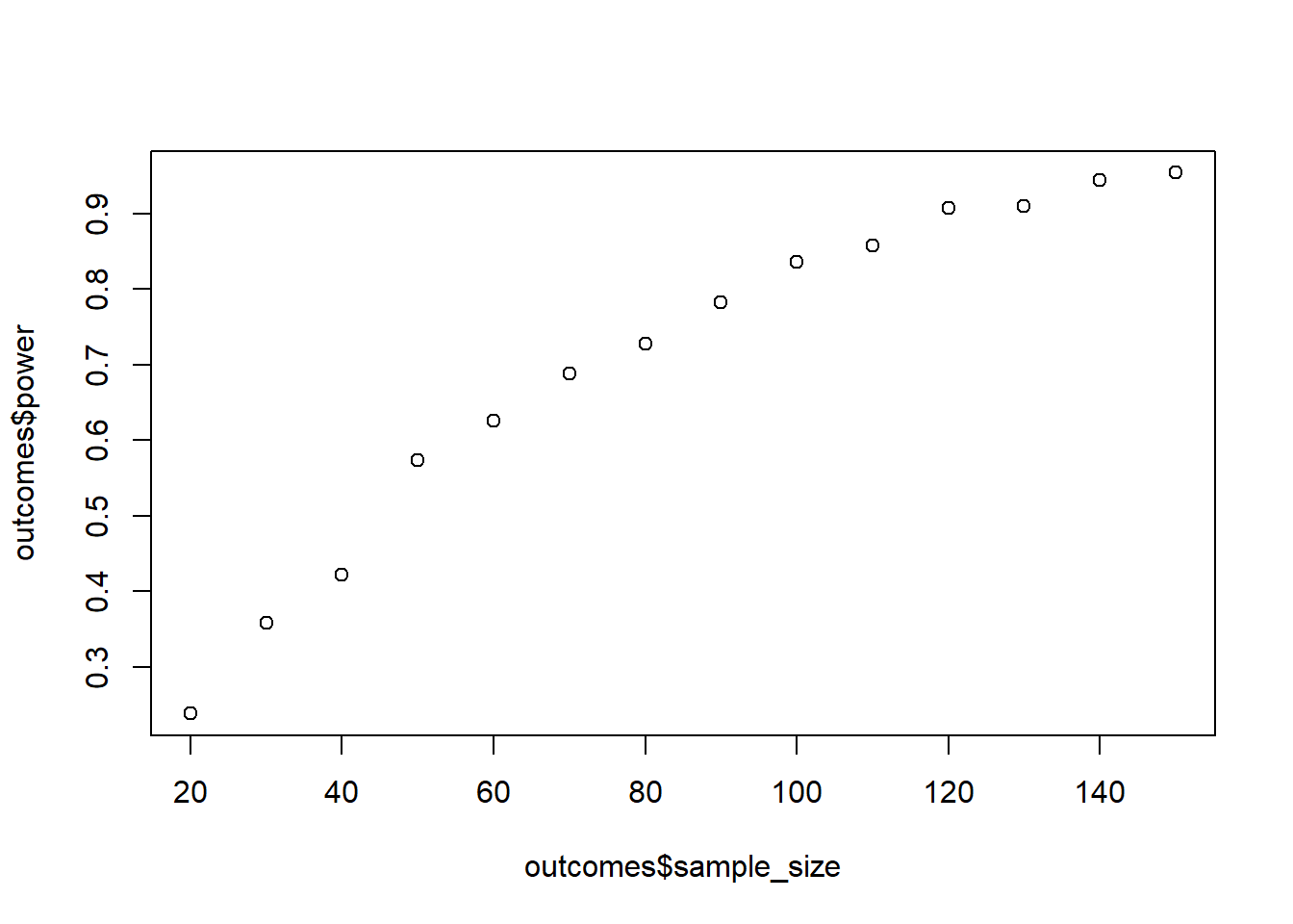
Expand to get a tip
I guess if this were a drinking game, you’d have to drink now: You have all the tools needed for this one. Let’s start with the stuff we know and declare our variables, define our variance-covariance matrix (which is easy because the SD is stable), and a place to store our results.
library(MASS)

sesoi <- ?
means <- c(none_low = ?, several_low = ?, none_high = ?, several_high = ? + sesoi)
sd <- ?
correlation <- ?
runs <- ?
sizes <- seq(?, ?, ?)

# get the covariance
covariance <- correlation * sd * sd

# put it all into our matrix
sigma <- matrix(
  c(
    sd**2, ?, ?, ?,
    ?, sd**2, ?, ?,
    ?, ?, ?, ?,
    ?, ?, ?, ?
  ),
  ncol = ?
)

# same as always
outcomes <-
  data.frame(
    sample_size = NULL,
    power = NULL
  )
The next step is getting the data into the right format. Ultimately, we want them to be in tidy (or long format), with one row per observation. With the below command, we can get the data into long format, but they won’t be ideal. Look at the condition variable.
pivot_longer(
  d,
  cols = -id,
  values_to = "scores",
  names_to = "condition"
)
# A tibble: 6 × 3
id condition scores
<fct> <chr> <dbl>
1 1 none_low 80.8
2 1 several_low 29.4
3 1 none_high 46.9
4 1 several_high 53.5
5 2 none_low 59.1
6 2 several_low 48.5They’ll need to somehow look like this:
# A tibble: 6 × 4
  id    Arguments Credibility scores
  <fct> <fct>     <fct>        <dbl>
1 1     none      low           80.8
2 1     several   low           29.4
3 1     none      high          46.9
4 1     several   high          53.5
5 2     none      low           59.1
6 2     several   low           48.5
You can create those two variables with an ifelse statement (or have a look at tidyr::separate). Once you have the data there, you just need to run the ANOVA and extract the p-value like we always do.
0.7 Exercise
You have a natural experiment coming up because you know that some users in the UK get a new streaming service before users in France. You want to know whether access to another streaming service increases satisfaction with people’s media diet. From the waiting list for that streaming service, you want to sample comparable users in the UK and France, ask them how satisfied they are with their media variety, wait for a month to give the UK users time to try out the new streaming service whereas the French users will be the control group. In other words, you have a mixed design with a pre-post measure within, but condition aka country (access to streaming) between.
You need to run a power analysis. For your measure of satisfaction, you use a 7-point Likert-scale. You assume that France at the pre-measure will score above the midpoint, given how many providers are already out there, say 3.9. You also expect no change, maybe even a slight decline seeing how the UK is getting access, so you set the post-measure to 3.8. For the UK, you expect a somewhat higher satisfaction already at pre-measure because they usually get stuff directly after the US, say 4.3. Importantly, you believe access to this new streaming service will increase satisfaction by 0.4 points–that’s the mimimum amount of change on that measure that predicts more users in the future. As for the SDs: You don’t see any reason why variation would increase from pre- to post-measure. However, you do believe there’s a bit more variation in France than in the UK based on previous research with large samples. You set the SD for France to 1.2, but for the UK to 0.9. As for correlations between pre- and post-measures: You expect France to be more consistent (0.6) than the UK (0.4).
Simulate power. You’ll need to do a variance-covariance matrix for correlated measures for each country (the within part) and then combine the two data frames (the between part). Base your power analysis on the interaction effect, not the simple effects. To run the ANOVA, you’ll need to properly nest the error, meaning Error(id/Time) in the aov_car command. You set your alpha to 0.01 and want to stop at 90% power. Start at 100 people per country and go up in steps of 20.
library(MASS)

set.seed(42)

means_france <- c(pre = 3.8, post = 3.9)
sd_france <- 1.2
cor_france <- 0.6
cov_france <- cor_france * sd_france * sd_france
means_uk <- c(pre = 4.3, post = 4.7)
sd_uk <- 0.9
cor_uk <- 0.4
cov_uk <- cor_uk * sd_uk * sd_uk
alpha <- 0.01
n <- 100
runs <- 500

sigma_france <-
  matrix(
    c(
      sd_france**2, cov_france,
      cov_france, sd_france**2
    ),
    ncol = 2
  )

sigma_uk <-
  matrix(
    c(
      sd_uk**2, cov_uk,
      cov_uk, sd_uk**2
    ),
    ncol = 2
  )

outcomes <-
  data.frame(
    sample_size = NULL,
    power = NULL
  )

power <- 0

while (power < 0.90) {

  pvalues <- NULL

  for (i in 1:runs) {

    france <- mvrnorm(
      n,
      means_france,
      sigma_france
    )

    france <- as.data.frame(france)
    france$country <- factor("france")
    france$id <- 1:n

    uk <- mvrnorm(
      n,
      means_uk,
      sigma_uk
    )

    uk <- as.data.frame(uk)
    uk$country <- factor("uk")
    uk$id <- (n+1):(2*n)

    d <- rbind(france, uk)

    d <- d %>%
      pivot_longer(
        cols = c(pre, post),
        names_to = "time",
        values_to = "satisfaction"

      )

    m <- suppressMessages(summary(afex::aov_car(satisfaction ~ country*time + Error(id/time), d), type = 3))

    pvalues[i] <- as.numeric(unlist(m)[26])
  }

  power <- sum(pvalues < alpha) / length(pvalues)

  outcomes <-
    rbind(
      outcomes,
      data.frame(
        sample_size = n,
        power = power
      )
    )

  n <- n + 20
}

plot(outcomes$sample_size, outcomes$power)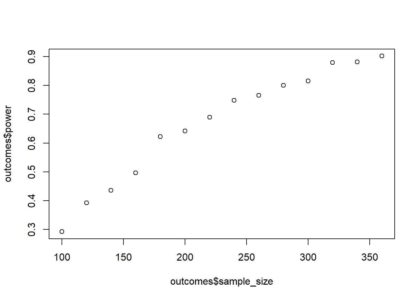
Expand to get a tip
I’m going to keep tips to a minimum here. Once you have everything declared, the rest should fall into place:
library(MASS)

means_france <- c(pre = ?, post = ?)
sd_france <- 1?
cor_france <- ? # correlation between measures for france
cov_france <- ? # covariance for france

means_uk <- c(pre = ?, post = ?)
sd_uk <- ?
cor_uk <- ?
cov_uk <- ?

alpha <- ?
n <- ?
runs <- ?

sigma_france <-
  matrix(
    ?
  )

sigma_uk <-
  matrix(
    ?
  )